我们已经分析了 Somatic mutations,并进行了注释和可视化,接下来我们进行拷贝数变异的分析。
这里我们还是先从 GATK 的 somatic cnv 的最佳实践开始
拷贝数变异(copy number variations, CNVs)是属于基因组结构变异(structural variation, SV),是指 DNA 片 段长度在 1Kb-3Mb 的基因组结构变异。我们首先从 GATK 的 CNV 流程开始 CNV 的分析。
首先是流程图,先从 bam 文件,结合坐标文件计算每个外显子的 reads counts 数,然后 call segment,最后是画图:
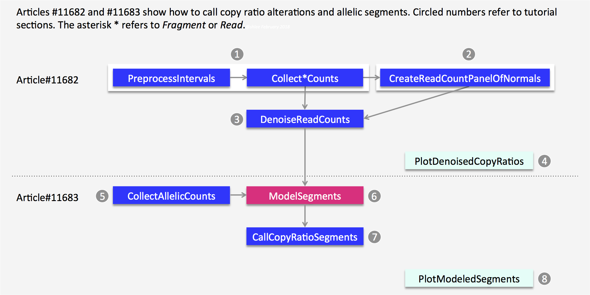
在下面这个链接中,给出了详细的教程:https://gatkforums.broadinstitute.org/gatk/discussion/11682#2
或者最近更新的教程,一样的:https://gatk.broadinstitute.org/hc/en-us/articles/360035531092
1. 外显子坐标的interval文件
interval 文件其实也是一个坐标文件,类似 bed,只不过 bed 文件的坐标是从 0 开始记录,而 interval 文件的坐标是从1开始记录。使用基因组 interval 文件可以定义软件分析的分辨率。如果是全基因组测序,interval 文件就用全基因组坐标的等间隔区间就好。对于外显子组的数据,我们使用捕获试剂盒的目标区域,理论上应该返回原文查找对应试剂盒,去搜索其捕获外显子的区域,一般是外显子侧翼上下游 250bp 以内。我懒得去查,就用软件的默认参数 250bp。
首先使用 BedToIntervalList 工具将 bed 转成 interval 格式(其实前面已经完成),然后用PreprocessIntervals工具获取 target 区间,即外显子侧翼上下游 250bp。
GATK=~/wes_cancer/biosoft/gatk-4.1.4.1/gatkref=~/wes_cancer/data/Homo_sapiens_assembly38.fastabed=~/wes_cancer/data/hg38.exon.beddict=~/wes_cancer/data/Homo_sapiens_assembly38.dict## bed to intervals_list$GATK BedToIntervalList -I ${bed} -O ~/wes_cancer/data/hg38.exon.interval_list -SD ${dict}## Preprocess Intervals$GATK PreprocessIntervals \-L ~/wes_cancer/data/hg38.exon.interval_list \--sequence-dictionary ${dict} \--reference ${ref} \--padding 250 \--bin-length 0 \--interval-merging-rule OVERLAPPING_ONLY \--output ~/wes_cancer/data/targets.preprocessed.interval.list
2. 获取样本的read counts
这里分为两小步进行:
- 首先是获取所有样本的 read counts,用到了工具是
CollectReadCounts,其根据所提供的 interval 文件,对 bam 文件进行 reads 计数,可以简单理解为把 bam 文件转换成 interval 区间的 reads 数。最后会生成一个 HDF5 格式的文件,需要用第三方软件 HDFView 来查看,这里不做展示。这个文件记录了每个基因组interval 文件的 CONTIG,START,END 和原始 COUNT 值,并制成表格。 - 然后构建正常样本的
CNV panel of normals,生成正常样本的cnvponM.pon.hdf5文件。对于外显子组捕获测序数据,捕获过程会引入一定的的噪音。因此后面需要降噪,该文件就是用于后面第 3 步DenoiseReadCounts。
实际使用到的脚本如下:
interval=~/wes_cancer/data/targets.preprocessed.interval.listGATK=~/wes_cancer/biosoft/gatk-4.1.4.1/gatkref=~/wes_cancer/data/Homo_sapiens_assembly38.fastacat config3 | while read iddoi=./5.gatk/${id}_bqsr.bamecho ${i}## step1 : CollectReadCountstime $GATK --java-options "-Xmx20G -Djava.io.tmpdir=./" CollectReadCounts \-I ${i} \-L ${interval} \-R ${ref} \--format HDF5 \--interval-merging-rule OVERLAPPING_ONLY \--output ./8.cnv/gatk/counts/${id}.clean_counts.hdf5## step2 : Generate a CNV panel of normals:cnvponM.pon.hdf5$GATK --java-options "-Xmx20G -Djava.io.tmpdir=./" CreateReadCountPanelOfNormals \--minimum-interval-median-percentile 5.0 \--output ./8.cnv/gatk/cnvponM.pon.hdf5 \--input ./8.cnv/gatk/counts/case1_germline.clean_counts.hdf5 \--input ./8.cnv/gatk/counts/case2_germline.clean_counts.hdf5 \--input ./8.cnv/gatk/counts/case3_germline.clean_counts.hdf5 \--input ./8.cnv/gatk/counts/case4_germline.clean_counts.hdf5 \--input ./8.cnv/gatk/counts/case5_germline.clean_counts.hdf5 \--input ./8.cnv/gatk/counts/case6_germline.clean_counts.hdf5done
这里的 input 重复了 6 次,为的是想让初学者容易理解。如果追求代码整洁,可以把这 6 句改成
$(for i in {1..6} ;do echo "--input ./8.cnv/gatk/counts/case${i}_germline.clean_counts.hdf5" ;done)
3. 降噪DenoiseReadCounts
该步骤用到的工具是 DenoiseReadCounts,主要是做了一个标准化和降噪,会生成两个文件 ${id}.clean.standardizedCR.tsv 和 ${id}.clean.denoisedCR.tsv,该工具会根据 PoN 的 counts 中位数对输入文件 ${id}.clean_counts.hdf5 进行一个标准化,包括 log2 转换。然后使用 PoN 的主成分进行标准化后的 copy ratios 降噪。实际上这里只需要对 tumor 样本进行降噪的,为了比较,我就把 tumor 和 normal 样本都分析了一遍,后面可以做个对比。
GATK=~/wes_cancer/biosoft/gatk-4.1.4.1/gatkcat config3 | while read iddoi=./8.cnv/gatk/counts/${id}.clean_counts.hdf5$GATK --java-options "-Xmx20g" DenoiseReadCounts \-I ${i} \--count-panel-of-normals ./8.cnv/gatk/cnvponM.pon.hdf5 \--standardized-copy-ratios ./8.cnv/gatk/standardizedCR/${id}.clean.standardizedCR.tsv \--denoised-copy-ratios ./8.cnv/gatk/denoisedCR/${id}.clean.denoisedCR.tsvdone
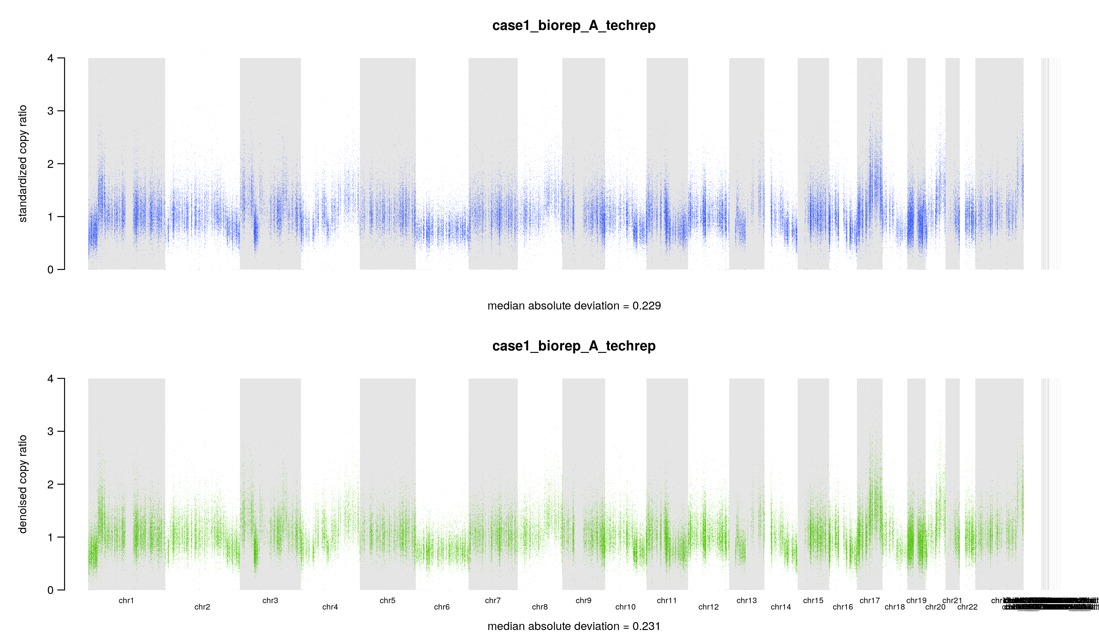
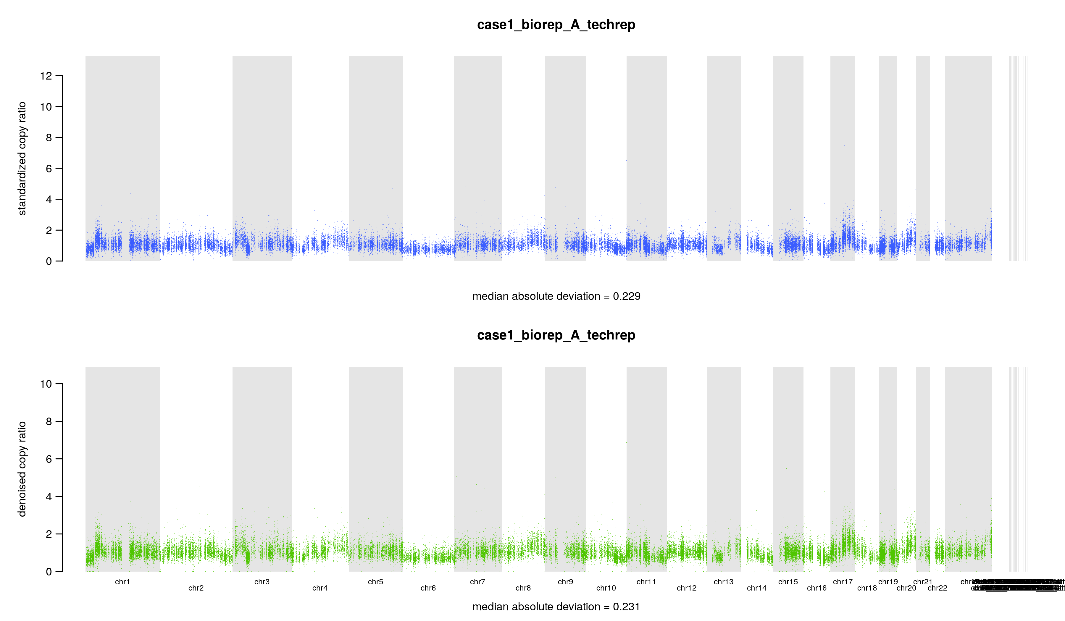
4. 可视化降噪后的copy ratios
我们使用 PlotDenoisedCopyRatios 可视化标准化和去噪的 read counts。这些图可以直观地评估去噪的效果。
GATK=~/wes_cancer/biosoft/gatk-4.1.4.1/gatkdict=~/wes_cancer/data/Homo_sapiens_assembly38.dictcat config3 | while read iddo$GATK --java-options "-Xmx20g" PlotDenoisedCopyRatios \--standardized-copy-ratios ./8.cnv/gatk/standardizedCR/${id}.clean.standardizedCR.tsv \--denoised-copy-ratios ./8.cnv/gatk/denoisedCR/${id}.clean.denoisedCR.tsv \--sequence-dictionary ${dict} \--output ./8.cnv/gatk/cnv_plots \--output-prefix ${id}done
对于每一个样本,如 case1_biorep_A_techrep,将生成 6 个文件:
./8.cnv/gatk/cnv_plots/case1_biorep_A_techrep.denoised.png./8.cnv/gatk/cnv_plots/case1_biorep_A_techrep.denoisedLimit4.png./8.cnv/gatk/cnv_plots/case1_biorep_A_techrep.deltaMAD.txt./8.cnv/gatk/cnv_plots/case1_biorep_A_techrep.scaledDeltaMAD.txt./8.cnv/gatk/cnv_plots/case1_biorep_A_techrep.standardizedMAD.txt./8.cnv/gatk/cnv_plots/case1_biorep_A_techrep.denoisedMAD.txt
其中4个文件是文本文件,里面就是一个数字,记录几个拷贝数变化比值 copy ratio 的中位数绝对偏差(median absolute deviation, MAD)
## 标准化后的 copy ratios 的 MAD$ cat ./8.cnv/gatk/cnv_plots/case1_biorep_A_techrep.standardizedMAD.txt0.229## 降噪后的 copy ratios 的 MAD$ cat ./8.cnv/gatk/cnv_plots/case1_biorep_A_techrep.denoisedMAD.txt0.231## 标准化后的 MAD 和降噪后的 MAD 的差$ cat ./8.cnv/gatk/cnv_plots/case1_biorep_A_techrep.deltaMAD.txt-0.002## (降噪后的 MAD - 标准化后的 MAD ) / (标准化后的 MAD )$ cat ./8.cnv/gatk/cnv_plots/case1_biorep_A_techrep.scaledDeltaMAD.txt-0.01
另外两个文件是图片,表达同一个意思,标准化和降噪后的 copy ratios,底下还有中位数绝对偏差(median absolute deviation, MAD),只不过一张图片把 y 轴设置为 0 到 4。假如 tumor 样本的拷贝数没有发生变化,copy ratio 应该稳定在 1 附近。当然,要是发生了 CNV 事件,那应该就在 1 附近波动。
5. 计算常见的germline mutation位点
这一步用到了 CollectAllelicCounts 工具,对输入的 bam 文件,根据指定的 interval 区间,进行 germline mutation 的检测(仅仅是 SNPs 位点,不包括 INDELs ),并计算该位点覆盖的 reads 数,即该位点的测序深度。值得注意的是,该工具一个默认参数是 MAPQ 值大于 20 的 reads 才会被纳入计数,最后生成一个 tsv 文件。
GENOME=~/wes_cancer/data/Homo_sapiens_assembly38.fastaGATK=~/wes_cancer/biosoft/gatk-4.1.4.1/gatkinterval=~/wes_cancer/data/targets.preprocessed.interval.listcat config3 | while read iddoi=./5.gatk/${id}_bqsr.bamecho ${i}time $GATK --java-options "-Xmx20G -Djava.io.tmpdir=./" CollectAllelicCounts \-I ${i} \-L ${interval} \-R ${GENOME} \-O ./8.cnv/gatk/allelicCounts/${id}.allelicCounts.tsvdone
生成的 tsv 文件主要内容如下(这里我过滤掉了第六列为 N 的位点):
$ less ./8.cnv/gatk/allelicCounts/case1_biorep_A_techrep.allelicCounts.tsv | grep -v ^@ | awk '{if($6 != "N") print $0}' |lessCONTIG POSITION REF_COUNT ALT_COUNT REF_NUCLEOTIDE ALT_NUCLEOTIDEchr1 925873 34 1 G Tchr1 925918 71 1 G Tchr1 925938 92 1 G Tchr1 925953 92 1 G Tchr1 925974 96 1 G Tchr1 925979 102 2 G A
6. ModelSegments
在第 3 步我们拿到了标准化和降噪后的两个 tsv 文件,记录了某个区间的 LOG2_COPY_RATIO 值,内容大致如下:
$ less ./8.cnv/gatk/denoisedCR/case1_biorep_A_techrep.clean.denoisedCR.tsv | grep -v ^@| lessCONTIG START END LOG2_COPY_RATIOchr1 925692 926262 -1.178123chr1 929905 930585 -0.569447chr1 930789 931338 -0.686712chr1 935522 936145 -0.404623chr1 938790 939201 -0.727205chr1 939202 939709 -0.882516
而第 5 步拿到的记录等位基因测序深度的 tsv 文件已经在上面展示过了。接下来第 6 步将利用这两个结果进行 call segment,需要注意的是输入文件要求 tumor match normal。不过好像也可以不输入第 5 步 CollectAllelicCounts 的结果,等有时间再比较一下两者的区别吧。这一步用到的工具是ModelSegments,它根据去噪后的第三步的 reads counts 值对 copy ratios 进行分割,并根据第五步的CollectAllelicCounts等位基因计数对分割片段进行分类。代码如下:
GATK=/~/wec_cancer/biosoft/gatk-4.1.4.1/gatkcat config3 | while read iddogermline=${id:0:5}_germline## ModelSegments$GATK --java-options "-Xmx20g" ModelSegments \--denoised-copy-ratios ./8.cnv/gatk/denoisedCR/${id}.clean.denoisedCR.tsv \--allelic-counts ./8.cnv/gatk/allelicCounts/${id}.allelicCounts.tsv \--normal-allelic-counts ./8.cnv/gatk/allelicCounts/${germline}.allelicCounts.tsv \--output ./8.cnv/gatk/segments \--output-prefix ${id}done
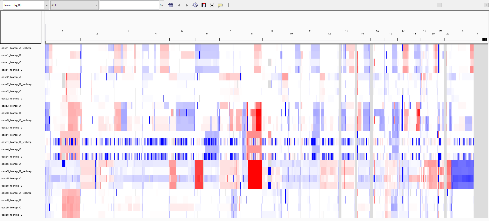
生成的文件有点多,每个样本生成 11 个文件。 param 文件包含用于 copy ratios(cr)和 allele fractions(af)的全局参数,而 seg 文件包含有关片段的数据。 具体说明可以查看这个链接:https://software.broadinstitute.org/gatk/documentation/tooldocs/4.1.4.0/org_broadinstitute_hellbender_tools_copynumber_ModelSegments.php
./8.cnv/gatk/segments/case1_biorep_A_techrep.af.igv.seg./8.cnv/gatk/segments/case1_biorep_A_techrep.cr.igv.seg./8.cnv/gatk/segments/case1_biorep_A_techrep.cr.seg./8.cnv/gatk/segments/case1_biorep_A_techrep.modelBegin.af.param./8.cnv/gatk/segments/case1_biorep_A_techrep.modelBegin.cr.param./8.cnv/gatk/segments/case1_biorep_A_techrep.modelBegin.seg./8.cnv/gatk/segments/case1_biorep_A_techrep.modelFinal.af.param./8.cnv/gatk/segments/case1_biorep_A_techrep.modelFinal.cr.param./8.cnv/gatk/segments/case1_biorep_A_techrep.modelFinal.seg./8.cnv/gatk/segments/case1_biorep_A_techrep.hets.normal.tsv./8.cnv/gatk/segments/case1_biorep_A_techrep.hets.tsv
其不过上面拿到的文件中的 ${id}*.igv.seg 文件,可以直接载入到 IGV 中进行可视化,如:
(不知道为什么,case4_biorep_B_techrep和case4_techrep_2的CNV事件是碎片化的,而 case5 病人的 X 染色体直接缺失)
7. CallCopyRatioSegments
这一步用来判断 copy ratio segments 是扩增、缺失、还是正常的可能性。对上一步拿到的${id}.cr.seg进行推断,得到${id}.clean.called.seg文件会增加一列 CALL,用 +、-、0分别表示扩增、缺失和正常。基本上MEAN_LOG2_COPY_RATIO大于 0.14 就是扩增,小于 -0.15 就是缺失,其他的为正常。
GATK=~/wes_cancer/biosoft/gatk-4.1.4.1/gatkcat config3 | while read iddo$GATK --java-options "-Xmx20g" CallCopyRatioSegments \-I ./8.cnv/gatk/segments/${id}.cr.seg \-O ./8.cnv/gatk/segments/${id}.clean.called.segdone
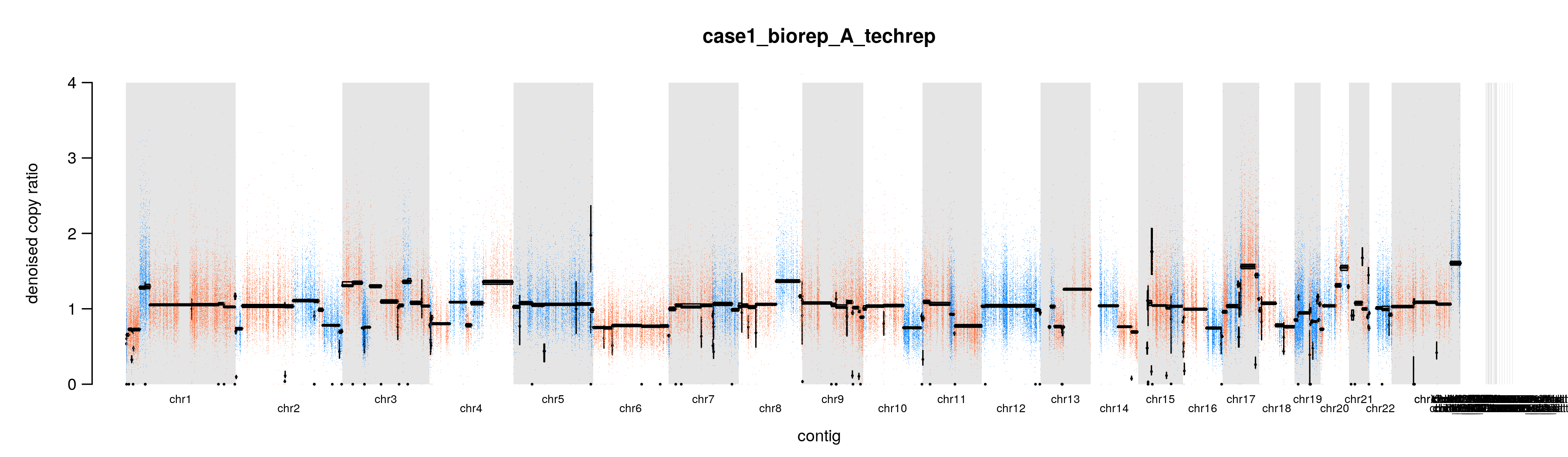
8. 可视化CNV结果
通过上面的分析,我们拿到了最后建模的 copy ratios 和 allele fractions segment,接下来用一个工具进行可视化:PlotModeledSegments
dict=~/wes_cancer/data/Homo_sapiens_assembly38.dictGATK=~/wes_cancer/biosoft/gatk-4.1.4.1/gatkcat config3 | while read iddo$GATK --java-options "-Xmx20g" PlotModeledSegments \--denoised-copy-ratios ./8.cnv/gatk/denoisedCR/${id}.clean.denoisedCR.tsv \--allelic-counts ./8.cnv/gatk/segments/${id}.hets.tsv \--segments ./8.cnv/gatk/segments/${id}.modelFinal.seg \--sequence-dictionary ${dict} \--output ./8.cnv/gatk/cnv_plots \--output-prefix ${id}.cleandone
整个gatk cnv流程
上面整个流程的代码,其实可以合并为一个脚本 gatk_cnv.sh:
GENOME=~/wes_cancer/data/Homo_sapiens_assembly38.fastadict=~/wes_cancer/data/Homo_sapiens_assembly38.dictINDEX=~/wes_cancer/data/bwa_index/gatk_hg38GATK=~/wes_cancer/biosoft/gatk-4.1.4.1/gatkDBSNP=~/wes_cancer/data/dbsnp_146.hg38.vcf.gzkgSNP=~/wes_cancer/data/1000G_phase1.snps.high_confidence.hg38.vcf.gzkgINDEL=~/wes_cancer/data/Mills_and_1000G_gold_standard.indels.hg38.vcf.gzinterval=~/wes_cancer/data/targets.preprocessed.interval.listcd ~/wes_cancer/project/8.cnv/gatk####################################### 把bam文件转为外显子reads数 #########################################cat ~/wes_cancer/project/config3 | while read iddoi=~/wes_cancer/project/5.gatk/${id}_bqsr.bamecho ${i}## step1 : CollectReadCountstime $GATK --java-options "-Xmx20G -Djava.io.tmpdir=./" CollectReadCounts \-I ${i} \-L ${interval} \-R ${GENOME} \--format HDF5 \--interval-merging-rule OVERLAPPING_ONLY \--output ${id}.clean_counts.hdf5## step2 : CollectAllelicCountstime $GATK --java-options "-Xmx20G -Djava.io.tmpdir=./" CollectAllelicCounts \-I ${i} \-L ${interval} \-R ${GENOME} \-O ${id}.allelicCounts.tsvdone### 注意这个CollectAllelicCounts步骤非常耗时,而且占空间mkdir allelicCountsmv *.allelicCounts.tsv ./allelicCountsmkdir countsmv *.clean_counts.hdf5 ./counts################################################### 接着合并所有的normal样本的数据创建 cnvponM.pon.hdf5 ###################################################$GATK --java-options "-Xmx20g" CreateReadCountPanelOfNormals \--minimum-interval-median-percentile 5.0 \--output cnvponM.pon.hdf5 \--input counts/case1_germline.clean_counts.hdf5 \--input counts/case2_germline.clean_counts.hdf5 \--input counts/case3_germline.clean_counts.hdf5 \--input counts/case4_germline.clean_counts.hdf5 \--input counts/case5_germline.clean_counts.hdf5 \--input counts/case6_germline.clean_counts.hdf5######################################################### 最后走真正的CNV流程 #########################################################cat config | while read iddoi=./counts/${id}.clean_counts.hdf5$GATK --java-options "-Xmx20g" DenoiseReadCounts \-I $i \--count-panel-of-normals cnvponM.pon.hdf5 \--standardized-copy-ratios ${id}.clean.standardizedCR.tsv \--denoised-copy-ratios ${id}.clean.denoisedCR.tsvdonemkdir denoisedCR standardizedCR segments cnv_plotsmv *denoisedCR.tsv ./denoisedCRmv *standardizedCR.tsv ./standardizedCRcat config | while read iddoi=./denoisedCR/${id}.clean.denoisedCR.tsv## ModelSegments的时候有两个策略,是否利用CollectAllelicCounts的结果$GATK --java-options "-Xmx20g" ModelSegments \--denoised-copy-ratios $i \--output segments \--output-prefix ${id}## 如果要利用CollectAllelicCounts的结果就需要增加两个参数,这里就不讲解了。$GATK --java-options "-Xmx20g" CallCopyRatioSegments \-I segments/${id}.cr.seg \-O segments/${id}.clean.called.seg## 这里面有两个绘图函数,PlotDenoisedCopyRatios 和 PlotModeledSegments ,可以选择性运行。$GATK --java-options "-Xmx20g" PlotDenoisedCopyRatios \--standardized-copy-ratios ./standardizedCR/${id}.clean.standardizedCR.tsv \--denoised-copy-ratios $i \--sequence-dictionary ${dict} \--output cnv_plots \--output-prefix ${id}$GATK --java-options "-Xmx20g" PlotModeledSegments \--denoised-copy-ratios $i \--segments segments/${id}.modelFinal.seg \--sequence-dictionary ${dict} \--output cnv_plots \--output-prefix ${id}.cleandone
对于每一个样本,就会拿到拷贝数变异的结果,如:


若有收获,就点个赞吧
0 人点赞
