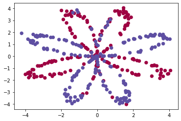
sklearn简单Logistic回归

在构建完整的神经网络之前，首先让我们看看逻辑回归在此问题上的表现。
你可以使用sklearn的内置函数来执行此操作。运行以下代码以在数据集上训练逻辑回归分类器。

# Train the logistic regression classifier
clf = sklearn.linear_model.LogisticRegressionCV();
clf.fit(X.T, Y.T);
# Plot the decision boundary for logistic regression
plot_decision_boundary(lambda x: clf.predict(x), X, Y)
plt.title("Logistic Regression")
# Print accuracy
LR_predictions = clf.predict(X.T)
print ('Accuracy of logistic regression: %d ' % float((np.dot(Y,LR_predictions) + np.dot(1-Y,1-LR_predictions))/float(Y.size)*100) +
       '% ' + "(percentage of correctly labelled datapoints)")

输出：Accuracy of logistic regression: 47 % (percentage of correctly labelled datapoints)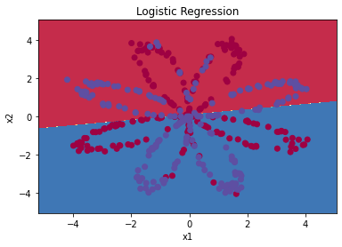

神经网络模型

从上面我们可以得知Logistic回归不适用于“flower数据集”。现在你将训练带有单个隐藏层的神经网络。
这是我们的模型：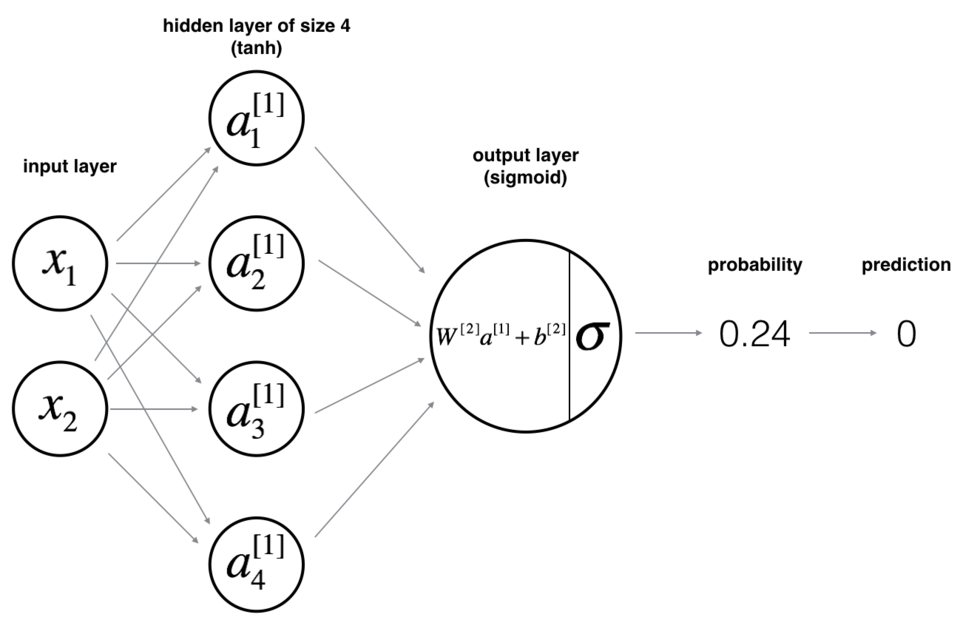

数学原理：

例如 $【HW】L1W3-单层神经网络 - 图4$ %7D#card=math&code=x%5E%7B%28i%29%7D&id=zAV90):

$【HW】L1W3-单层神经网络 - 图5$ %7D%20%3D%20%20W%5E%7B%5B1%5D%7D%20x%5E%7B(i)%7D%20%2B%20b%5E%7B%5B1%5D%20(i)%7D%5Ctag%7B1%7D%0A#card=math&code=z%5E%7B%5B1%5D%20%28i%29%7D%20%3D%20%20W%5E%7B%5B1%5D%7D%20x%5E%7B%28i%29%7D%20%2B%20b%5E%7B%5B1%5D%20%28i%29%7D%5Ctag%7B1%7D%0A&id=pe363)

$【HW】L1W3-单层神经网络 - 图6$ %7D%20%3D%20%5Ctanh(z%5E%7B%5B1%5D%20(i)%7D)%5Ctag%7B2%7D%0A#card=math&code=a%5E%7B%5B1%5D%20%28i%29%7D%20%3D%20%5Ctanh%28z%5E%7B%5B1%5D%20%28i%29%7D%29%5Ctag%7B2%7D%0A&id=Dd5KW)

$【HW】L1W3-单层神经网络 - 图7$ %7D%20%3D%20W%5E%7B%5B2%5D%7D%20a%5E%7B%5B1%5D%20(i)%7D%20%2B%20b%5E%7B%5B2%5D%20(i)%7D%5Ctag%7B3%7D%0A#card=math&code=z%5E%7B%5B2%5D%20%28i%29%7D%20%3D%20W%5E%7B%5B2%5D%7D%20a%5E%7B%5B1%5D%20%28i%29%7D%20%2B%20b%5E%7B%5B2%5D%20%28i%29%7D%5Ctag%7B3%7D%0A&id=dfztn)

$【HW】L1W3-单层神经网络 - 图8$ %7D%20%3D%20a%5E%7B%5B2%5D%20(i)%7D%20%3D%20%5Csigma(z%5E%7B%20%5B2%5D%20(i)%7D)%5Ctag%7B4%7D%0A#card=math&code=%5Chat%7By%7D%5E%7B%28i%29%7D%20%3D%20a%5E%7B%5B2%5D%20%28i%29%7D%20%3D%20%5Csigma%28z%5E%7B%20%5B2%5D%20%28i%29%7D%29%5Ctag%7B4%7D%0A&id=M7EIe)

$【HW】L1W3-单层神经网络 - 图9$ %7D%7Bprediction%7D%20%3D%20%5Cbegin%7Bcases%7D%201%20%26%20%5Cmbox%7Bif%20%7D%20a%5E%7B%5B2%5D(i)%7D%20%3E%200.5%20%5C%5C%200%20%26%20%5Cmbox%7Botherwise%20%7D%20%5Cend%7Bcases%7D%5Ctag%7B5%7D%0A#card=math&code=y%5E%7B%28i%29%7D%7Bprediction%7D%20%3D%20%5Cbegin%7Bcases%7D%201%20%26%20%5Cmbox%7Bif%20%7D%20a%5E%7B%5B2%5D%28i%29%7D%20%3E%200.5%20%5C%5C%200%20%26%20%5Cmbox%7Botherwise%20%7D%20%5Cend%7Bcases%7D%5Ctag%7B5%7D%0A&id=tnXFC)

根据所有的预测数据，你还可以如下计算损失 $【HW】L1W3-单层神经网络 - 图10$ :

$【HW】L1W3-单层神经网络 - 图11$ %7D%5Clog%5Cleft(a%5E%7B%5B2%5D%20(i)%7D%5Cright)%20%2B%20(1-y%5E%7B(i)%7D)%5Clog%5Cleft(1-%20a%5E%7B%5B2%5D%20(i)%7D%5Cright)%20%20%5Clarge%20%20%5Cright)%20%5Csmall%20%5Ctag%7B6%7D%0A#card=math&code=J%20%3D%20-%20%5Cfrac%7B1%7D%7Bm%7D%20%5Csum%5Climits_%7Bi%20%3D%200%7D%5E%7Bm%7D%20%5Clarge%5Cleft%28%5Csmall%20y%5E%7B%28i%29%7D%5Clog%5Cleft%28a%5E%7B%5B2%5D%20%28i%29%7D%5Cright%29%20%2B%20%281-y%5E%7B%28i%29%7D%29%5Clog%5Cleft%281-%20a%5E%7B%5B2%5D%20%28i%29%7D%5Cright%29%20%20%5Clarge%20%20%5Cright%29%20%5Csmall%20%5Ctag%7B6%7D%0A&id=qjowO)
建立神经网络的一般方法是：

定义神经网络结构（输入单元数，隐藏单元数等）；
初始化模型的参数；
循环：
1. 实现前向传播
2. 计算损失
3. 后向传播以获得梯度
4. 更新参数（梯度下降）

我们通常会构建辅助函数来计算第 a-c 步，然后将它们合并为nn_model()函数。一旦构建了nn_model()并学习了正确的参数，就可以对新数据进行预测。

1.定义神经网络结构

# 1.定义神经网络结构（输入单元数，隐藏单元数等）
# 定义三个变量： - n_x：输入层的大小 - n_h：隐藏层的大小（将其设置为4） - n_y：输出层的大小
def layer_sizes(X, Y):
    n_x = X.shape[0]
    n_h = 4
    n_y = Y.shape[0]
    return (n_x, n_h, n_y)

2.初始化模型的参数

# 2.初始化模型的参数，权重矩阵为随机值，偏差向量为0
def initialize_parameters(n_x, n_h, n_y):
    np.random.seed(2) # we set up a seed so that your output matches ours although the initialization is random.
    ### START CODE HERE ### (≈ 4 lines of code)
    W1 = np.random.randn(n_h, n_x) * 0.01
    W2 = np.random.randn(n_y, n_h) * 0.01
    b1 = np.zeros((n_h, 1))
    b2 = np.zeros((n_y, 1))
    ### END CODE HERE ###
    assert (W1.shape == (n_h, n_x))
    assert (b1.shape == (n_h, 1))
    assert (W2.shape == (n_y, n_h))
    assert (b2.shape == (n_y, 1))
    parameters = {"W1": W1,
                  "b1": b1,
                  "W2": W2,
                  "b2": b2}    
    return parameters
parameters = initialize_parameters(n_x, n_h, n_y)

3.循环

# 3.循环
def forward_propagation(X, parameters):
    # Retrieve each parameter from the dictionary "parameters"
    ### START CODE HERE ### (≈ 4 lines of code)
    W1 = parameters['W1']
    W2 = parameters['W2']
    b1 = parameters['b1']
    b2 = parameters['b2']
    ### END CODE HERE ###
    # Implement Forward Propagation to calculate A2 (probabilities)
    ### START CODE HERE ### (≈ 4 lines of code)
    Z1 = np.dot(W1, X) + b1
    A1 = np.tanh(Z1)
    Z2 = np.dot(W2, A1) + b2
    A2 = sigmoid(Z2)
    ### END CODE HERE ###
    assert(A2.shape == (1, X.shape[1]))
    cache = {"Z1": Z1,
             "A1": A1,
             "Z2": Z2,
             "A2": A2}
    return A2, cache
A2, cache = forward_propagation(X_assess, parameters)

计算损失函数如下：

$【HW】L1W3-单层神经网络 - 图12$ %7D%5Clog%5Cleft(a%5E%7B%5B2%5D%20(i)%7D%5Cright)%20%2B%20(1-y%5E%7B(i)%7D)%5Clog%5Cleft(1-%20a%5E%7B%5B2%5D%20(i)%7D%5Cright)%20%5Clarge%7B)%7D%20%5Csmall%0A#card=math&code=J%20%3D%20-%20%5Cfrac%7B1%7D%7Bm%7D%20%5Csum%5Climits_%7Bi%20%3D%200%7D%5E%7Bm%7D%20%5Clarge%7B%28%7D%20%5Csmall%20y%5E%7B%28i%29%7D%5Clog%5Cleft%28a%5E%7B%5B2%5D%20%28i%29%7D%5Cright%29%20%2B%20%281-y%5E%7B%28i%29%7D%29%5Clog%5Cleft%281-%20a%5E%7B%5B2%5D%20%28i%29%7D%5Cright%29%20%5Clarge%7B%29%7D%20%5Csmall%0A&id=ucZPG)

def compute_cost(A2, Y, parameters):
    m = Y.shape[1] # number of example
    # Compute the cross-entropy cost
    ### START CODE HERE ### (≈ 2 lines of code)
    logp = np.multiply(np.log(A2),Y) + np.multiply((1 - Y), np.log(1-A2))
    cost = -1/m * np.sum(logp)
    ### END CODE HERE ###
    cost = np.squeeze(cost)     # makes sure cost is the dimension we expect. 
                                # E.g., turns [[17]] into 17 
    assert(isinstance(cost, float))
    return cost
print("cost = " + str(compute_cost(A2, Y_assess, parameters)))

接下来实现反向传播，根据图中右侧的公式即可。

def backward_propagation(parameters, cache, X, Y):
    m = X.shape[1]
    W1 = parameters['W1']
    W2 = parameters['W2']
    A1 = cache["A1"]
    A2 = cache['A2']
    # Backward propagation: calculate dW1, db1, dW2, db2. 
    ### START CODE HERE ### (≈ 6 lines of code, corresponding to 6 equations on slide above)
    dZ2 = A2 - Y
    dW2 = 1/m * np.dot(dZ2, A1.T)
    db2 = 1/m * np.sum(dZ2, axis = 1, keepdims=True)
    dZ1 = np.dot(W2.T, dZ2) * (1 - np.power(A1, 2))
    dW1 = 1/m * np.dot(dZ1, X.T)
    db1 = 1/m * np.sum(dZ1, axis = 1, keepdims=True)
    ### END CODE HERE ###
    grads = {"dW1": dW1,
             "db1": db1,
             "dW2": dW2,
             "db2": db2}
    return grads
grads = backward_propagation(parameters, cache, X_assess, Y_assess)

# 更新参数
def update_parameters(parameters, grads, learning_rate = 1.2):
    W1 = parameters["W1"]
    b1 = parameters["b1"]
    W2 = parameters["W2"]
    b2 = parameters["b2"]
    dW1 = grads["dW1"]
    db1 = grads["db1"]
    dW2 = grads["dW2"]
    db2 = grads["db2"]
    # Update rule for each parameter
    ### START CODE HERE ### (≈ 4 lines of code)
    W1 = W1 - learning_rate * dW1
    b1 = b1 - learning_rate * db1
    W2 = W2 - learning_rate * dW2
    b2 = b2 - learning_rate * db2
    ### END CODE HERE ###
    parameters = {"W1": W1,
                  "b1": b1,
                  "W2": W2,
                  "b2": b2}
    return parameters
parameters = update_parameters(parameters, grads)

# 在 nn_model() 中集成上面的函数
def nn_model(X, Y, n_h, num_iterations = 10000, print_cost=False):
    np.random.seed(3)
    n_x = layer_sizes(X, Y)[0]
    n_y = layer_sizes(X, Y)[2]
    # Initialize parameters, then retrieve W1, b1, W2, b2. Inputs: "n_x, n_h, n_y". Outputs = "W1, b1, W2, b2, parameters".
    ### START CODE HERE ### (≈ 5 lines of code)
    parameters = initialize_parameters(n_x, n_h, n_y)
    b1 = parameters['b1']
    b2 = parameters['b2']
    W1 = parameters['W1']
    W2 = parameters['W2']
    ### END CODE HERE ###
    # Loop (gradient descent)
    for i in range(0, num_iterations):
        ### START CODE HERE ### (≈ 4 lines of code)
        A2, cache = forward_propagation(X, parameters)
        cost = compute_cost(A2, Y, parameters)
        grads = backward_propagation(parameters, cache, X, Y)
        parameters = update_parameters(parameters, grads, learning_rate = 1.2)
        ### END CODE HERE ###
        # Print the cost every 1000 iterations
        if print_cost and i % 1000 == 0:
            print ("Cost after iteration %i: %f" %(i, cost))
    return parameters
parameters = nn_model(X_assess, Y_assess, 4, num_iterations=10000, print_cost=False)

预测

# 使用正向传播来预测结果。
def predict(parameters, X):
    # Computes probabilities using forward propagation, and classifies to 0/1 using 0.5 as the threshold.
    ### START CODE HERE ### (≈ 2 lines of code)
    A2, cache = forward_propagation(X, parameters)
    predictions = np.round(A2)
    ### END CODE HERE ###
    return predictions
predictions = predict(parameters, X_assess)

现在运行模型以查看其如何在二维数据集上运行。运行以下代码以使用含有 𝑛_ℎ 隐藏单元的单个隐藏层测试模型。

# Build a model with a n_h-dimensional hidden layer
parameters = nn_model(X, Y, n_h = 4, num_iterations = 10000, print_cost=True)
# Plot the decision boundary
plot_decision_boundary(lambda x: predict(parameters, x.T), X, Y)
plt.title("Decision Boundary for hidden layer size " + str(4))
# Print accuracy
predictions = predict(parameters, X)
print ('Accuracy: %d' % float((np.dot(Y,predictions.T) + np.dot(1-Y,1-predictions.T))/float(Y.size)*100) + '%')

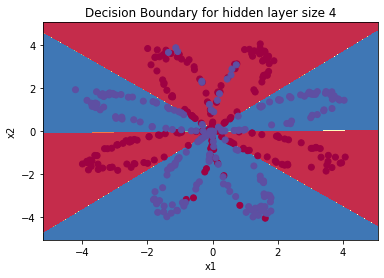
Accuracy: 90%