2. 正向传播
GRADED FUNCTION: L_model_forward
- 4. 反向传播
- 5. 更新参数
深度神经网络应用—图像分类

让我们首先导入作业过程中需要的所有包。

numpy是Python科学计算的基本包。
matplotlib是在Python中常用的绘制图形的库。
dnn_utils 为此笔记本提供了一些必要的函数。
testCases 提供了一些测试用例来评估函数的正确性
np.random.seed（1）使所有随机函数调用保持一致。这将有助于我们评估你的作业，请不要改变seed。 ```python import numpy as np import h5py import matplotlib.pyplot as plt from testCases_v2 import * from dnn_utils_v2 import sigmoid, sigmoid_backward, relu, relu_backward

%matplotlib inline plt.rcParams[‘figure.figsize’] = (5.0, 4.0) # set default size of plots plt.rcParams[‘image.interpolation’] = ‘nearest’ plt.rcParams[‘image.cmap’] = ‘gray’

%load_ext autoreload %autoreload 2

np.random.seed(1)

<a name="fGC5j"></a>
# 逐步构建深度神经网络
<a name="GGJpo"></a>
## 0 作业大纲
1. 初始化神经网络的参数。
2. 实现正向传播模块（在下图中以紫色显示）。 
   - 完成模型正向传播步骤的LINEAR部分（）。
   - 提供使用的ACTIVATION函数（relu / Sigmoid）。
   - 将前两个步骤合并为新的[LINEAR-> ACTIVATION]前向函数。
   - 堆叠[LINEAR-> RELU]正向函数L-1次（第1到L-1层），并在末尾添加[LINEAR-> SIGMOID]（最后的层）。这合成了一个新的L_model_forward函数。
3. 计算损失。
4. 实现反向传播模块（在下图中以红色表示）。 
   - 完成模型反向传播步骤的LINEAR部分。
   - 提供的ACTIVATE函数的梯度（relu_backward / sigmoid_backward）
   - 将前两个步骤组合成新的[LINEAR-> ACTIVATION]反向函数。
   - 将[LINEAR-> RELU]向后堆叠L-1次，并在新的L_model_backward函数中后向添加[LINEAR-> SIGMOID]
5. 最后更新参数。
<a name="VqT22"></a>
## 1. L层初始化
- 模型的结构为 _[LINEAR -> RELU]  * (L-1) -> LINEAR -> SIGMOID_。也就是说，前![](https://g.yuque.com/gr/latex?L-1#card=math&code=L-1&id=eHfpf)层使用ReLU作为激活函数，最后一层采用sigmoid激活函数输出。
- 随机初始化权重矩阵。使用`np.random.rand（shape）* 0.01`。
- 零初始化偏差。使用`np.zeros（shape）`。
- 我们将在不同的layer_dims变量中存储![](https://g.yuque.com/gr/latex?n%5E%7B%5Bl%5D%7D#card=math&code=n%5E%7B%5Bl%5D%7D&id=dkYlp)，即不同层中的神经元数。例如，上周“二维数据分类模型”的`layer_dims`为[2,4,1]：即有两个输入，一个隐藏层包含4个隐藏单元，一个输出层包含1个输出单元。因此，`W1`的维度为（4,2），`b1`的维度为（4,1），`W2`的维度为（1,4），而`b2`的维度为（1,1）。现在你将把它应用到![](https://g.yuque.com/gr/latex?L#card=math&code=L&id=r28X2)层！
```python
def initialize_parameters_deep(layer_dims):
    np.random.seed(3)
    parameters = {}
    L = len(layer_dims)            # number of layers in the network
    for l in range(1, L):
        parameters['W' + str(l)] = np.random.randn(layer_dims[l], layer_dims[l-1]) * 0.01
        parameters['b' + str(l)] = np.zeros((layer_dims[l], 1))
        assert(parameters['W' + str(l)].shape == (layer_dims[l], layer_dims[l-1]))
        assert(parameters['b' + str(l)].shape == (layer_dims[l], 1))
    return parameters
parameters = initialize_parameters_deep([5,4,3])

{'W1': array([[ 0.01788628,  0.0043651 ,  0.00096497, -0.01863493, -0.00277388],
        [-0.00354759, -0.00082741, -0.00627001, -0.00043818, -0.00477218],
        [-0.01313865,  0.00884622,  0.00881318,  0.01709573,  0.00050034],
        [-0.00404677, -0.0054536 , -0.01546477,  0.00982367, -0.01101068]]),
 'b1': array([[0.],
        [0.],
        [0.],
        [0.]]),
 'W2': array([[-0.01185047, -0.0020565 ,  0.01486148,  0.00236716],
        [-0.01023785, -0.00712993,  0.00625245, -0.00160513],
        [-0.00768836, -0.00230031,  0.00745056,  0.01976111]]),
 'b2': array([[0.],
        [0.],
        [0.]])}

2. 正向传播

2.1 线性正向

现在，你已经初始化了参数，接下来将执行正向传播模块。首先实现一些基本函数，用于稍后的模型实现。按以下顺序完成三个函数：

LINEAR
LINEAR -> ACTIVATION，其中激活函数采用ReLU或Sigmoid。
[LINEAR -> RELU] $【HW】L1W4-深度神经网络 - 图1$ (L-1) -> LINEAR -> SIGMOID（整个模型）

线性正向模块（在所有数据中均进行向量化）的计算按照以下公式：
$【HW】L1W4-深度神经网络 - 图2$
其中 $【HW】L1W4-深度神经网络 - 图3$ .

练习：建立正向传播的线性部分。
提醒：
该单元的数学表示为 $【HW】L1W4-深度神经网络 - 图4$ ，你可能会发现np.dot（）有用。如果维度不匹配，则可以printW.shape查看修改。

[LINEAR -> RELU] $【HW】L1W4-深度神经网络 - 图5$ (L-1) -> LINEAR -> SIGMOID（整个模型）

# GRADED FUNCTION: linear_forward
def linear_forward(A, W, b):
    Z = np.dot(W, A) + b
    assert(Z.shape == (W.shape[0], A.shape[1]))
    cache = (A, W, b)
    return Z, cache
A, W, b = linear_forward_test_case()
Z, linear_cache = linear_forward(A, W, b)

就是进行一个线性计算Z = np.dot(W, A) + b

2.2 正向线性激活

在此笔记本中，你将使用两个激活函数：

Sigmoid： $【HW】L1W4-深度神经网络 - 图6$ %20%3D%20%5Csigma(W%20A%20%2B%20b)%20%3D%20%5Cfrac%7B1%7D%7B%201%20%2B%20e%5E%7B-(W%20A%20%2B%20b)%7D%7D#card=math&code=%5Csigma%28Z%29%20%3D%20%5Csigma%28W%20A%20%2B%20b%29%20%3D%20%5Cfrac%7B1%7D%7B%201%20%2B%20e%5E%7B-%28W%20A%20%2B%20b%29%7D%7D&id=KfiqS)。我们为你提供了“ Sigmoid”函数。该函数返回两项值：激活值”a“和包含”Z“的”cache“（这是我们将馈入到相应的反向函数的内容）。
ReLU：ReLu的数学公式为 $【HW】L1W4-深度神经网络 - 图7$ %20%3D%20max(0%2C%20Z)#card=math&code=A%20%3D%20RELU%28Z%29%20%3D%20max%280%2C%20Z%29&id=lnFll)。我们为你提供了relu函数。该函数返回两项值：激活值“A”和包含“Z”的“cache”（这是我们将馈入到相应的反向函数的内容）。 ```python def sigmoid(Z): A = 1/(1+np.exp(-Z)) cache = Z

return A, cache

def relu(Z): A = np.maximum(0,Z)

assert(A.shape == Z.shape)
cache = Z 
return A, cache


```python
# GRADED FUNCTION: linear_activation_forward
def linear_activation_forward(A_prev, W, b, activation):
    if activation == "sigmoid":
        # Inputs: "A_prev, W, b". Outputs: "A, activation_cache".
        Z, linear_cache = linear_forward(A_prev,W,b)
        A, activation_cache = sigmoid(Z)
    elif activation == "relu":
        # Inputs: "A_prev, W, b". Outputs: "A, activation_cache".
        Z, linear_cache = linear_forward(A_prev,W,b)
        A, activation_cache = relu(Z)
    assert (A.shape == (W.shape[0], A_prev.shape[1]))
    cache = (linear_cache, activation_cache)
    return A, cache

就是对线性计算套了一层非线性计算，可选relu或者 sigmoid。

4.3 L层模型

为了方便实现 $【HW】L1W4-深度神经网络 - 图8$ 层神经网络，你将需要一个函数来复制前一个函数（使用RELU的linear_activation_forward） $【HW】L1W4-深度神经网络 - 图9$ 次，以及复制带有SIGMOID的linear_activation_forward。

练习：实现上述模型的正向传播。
说明：在下面的代码中，变量AL表示 $【HW】L1W4-深度神经网络 - 图10$ %20%3D%20%5Csigma(W%5E%7B%5BL%5D%7D%20A%5E%7B%5BL-1%5D%7D%20%2B%20b%5E%7B%5BL%5D%7D)#card=math&code=A%5E%7B%5BL%5D%7D%20%3D%20%5Csigma%28Z%5E%7B%5BL%5D%7D%29%20%3D%20%5Csigma%28W%5E%7B%5BL%5D%7D%20A%5E%7B%5BL-1%5D%7D%20%2B%20b%5E%7B%5BL%5D%7D%29&id=U9sl8)（有时也称为Yhat，即 $【HW】L1W4-深度神经网络 - 图11$ 。）
提示：

使用你先前编写的函数
使用for循环复制[LINEAR-> RELU]（L-1）次
不要忘记在“cache”列表中更新缓存。要将新值 c添加到list中，可以使用list.append(c)。 ```python
GRADED FUNCTION: L_model_forward

def L_model_forward(X, parameters): “”” X — data, numpy array of shape (input size, number of examples) parameters — output of initialize_parameters_deep() AL — last post-activation value caches — list of caches containing: every cache of linear_relu_forward() (there are L-1 of them, indexed from 0 to L-2) the cache of linear_sigmoid_forward() (there is one, indexed L-1) “””

caches = []
A = X
L = len(parameters) // 2                  # number of layers in the neural network
# Implement [LINEAR -> RELU]*(L-1). Add "cache" to the "caches" list.
for l in range(1, L):
    A_prev = A 
    A, linear_activation_cache = linear_activation_forward(A_prev, parameters['W' + str(l)], parameters['b' + str(l)], activation = "relu")
    caches.append(linear_activation_cache)
# Implement LINEAR -> SIGMOID. Add "cache" to the "caches" list.
AL, linear_activation_cache = linear_activation_forward(A, parameters['W' + str(L)], parameters['b' + str(L)], activation = "sigmoid")
caches.append(linear_activation_cache)
assert(AL.shape == (1,X.shape[1]))
return AL, caches

X, parameters = L_model_forward_test_case() AL, caches = L_model_forward(X, parameters) print(X,’\n’, parameters,’\nAL = ‘, AL,’\n caches = \n’, caches)

[[ 1.62434536 -0.61175641] [-0.52817175 -1.07296862] [ 0.86540763 -2.3015387 ] [ 1.74481176 -0.7612069 ]] {‘W1’: array([[ 0.3190391 , -0.24937038, 1.46210794, -2.06014071], [-0.3224172 , -0.38405435, 1.13376944, -1.09989127], [-0.17242821, -0.87785842, 0.04221375, 0.58281521]]), ‘b1’: array([[-1.10061918], [ 1.14472371], [ 0.90159072]]), ‘W2’: array([[ 0.50249434, 0.90085595, -0.68372786]]), ‘b2’: array([[-0.12289023]])} AL = [[0.17007265 0.2524272 ]] caches = [((array([[ 1.62434536, -0.61175641], [-0.52817175, -1.07296862], [ 0.86540763, -2.3015387 ]]), array([[ 1.74481176, -0.7612069 , 0.3190391 ]]), array([[-0.24937038]])), array([[-2.77991749, -2.82513147], [-0.11407702, -0.01812665], [ 2.13860272, 1.40818979]])), ((array([[ 1.62434536, -0.61175641], [-0.52817175, -1.07296862], [ 0.86540763, -2.3015387 ]]), array([[ 1.74481176, -0.7612069 , 0.3190391 ]]), array([[-0.24937038]])), array([[-1.58511248, -1.08570881]]))]

就是加了层循环嘛，有几层网络就循环几次。
<a name="7162a4e0"></a>
## 3. 损失函数
使用以下公式计算交叉熵损失![](https://g.yuque.com/gr/latex?J#card=math&code=J&id=oRuzv)：
![](https://g.yuque.com/gr/latex?-%5Cfrac%7B1%7D%7Bm%7D%20%5Csum%5Climits_%7Bi%20%3D%201%7D%5E%7Bm%7D%20(y%5E%7B(i)%7D%5Clog%5Cleft(a%5E%7B%5BL%5D%20(i)%7D%5Cright)%20%2B%20(1-y%5E%7B(i)%7D)%5Clog%5Cleft(1-%20a%5E%7B%5BL%5D(i)%7D%5Cright))%C2%A0%5Ctag%7B7%7D%0A#card=math&code=-%5Cfrac%7B1%7D%7Bm%7D%20%5Csum%5Climits_%7Bi%20%3D%201%7D%5E%7Bm%7D%20%28y%5E%7B%28i%29%7D%5Clog%5Cleft%28a%5E%7B%5BL%5D%20%28i%29%7D%5Cright%29%20%2B%20%281-y%5E%7B%28i%29%7D%29%5Clog%5Cleft%281-%20a%5E%7B%5BL%5D%28i%29%7D%5Cright%29%29%C2%A0%5Ctag%7B7%7D%0A&id=JlHvV)
```python
# GRADED FUNCTION: compute_cost
def compute_cost(AL, Y):  
    m = Y.shape[1]
    # Compute loss from aL and y.
    cost = - 1/m * np.sum(Y * np.log(AL) + (1 - Y) * np.log(1 - AL), axis=1, keepdims=True)
    cost = np.squeeze(cost)      # To make sure your cost's shape is what we expect (e.g. this turns [[17]] into 17).
    assert(cost.shape == ())
    return cost

4. 反向传播

4.1 线性反向

请记住，反向传播用于计算损失函数相对于参数的梯度。
对于层 $【HW】L1W4-深度神经网络 - 图12$ ，线性部分为： $【HW】L1W4-深度神经网络 - 图13$ （之后是激活）。

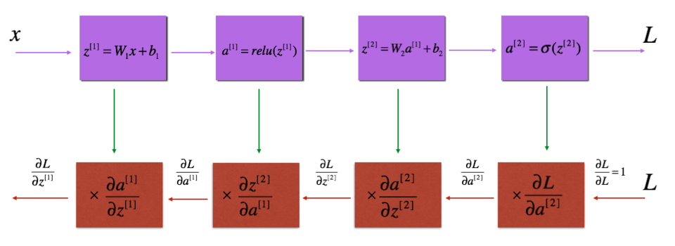
图：LINEAR->RELU->LINEAR->SIGMOID 的正向和反向传播，紫色块代表正向传播，红色块代表反向传播。

类似于正向传播，你将分三个步骤构建反向传播：
LINEAR backward
LINEAR -> ACTIVATION backward，其中激活函数使用ReLU或sigmoid 的导数计算
[LINEAR -> RELU] × (L-1) -> LINEAR -> SIGMOID backward（整个模型）

假设你已经计算出导数 $【HW】L1W4-深度神经网络 - 图15$ 。你想获得 $【HW】L1W4-深度神经网络 - 图16$ #card=math&code=%28dW%5E%7B%5Bl%5D%7D%2C%20db%5E%7B%5Bl%5D%7D%20dA%5E%7B%5Bl-1%5D%7D%29&id=cb4qM)。
使用输入 $【HW】L1W4-深度神经网络 - 图17$ 计算三个输出 $【HW】L1W4-深度神经网络 - 图18$ #card=math&code=%28dW%5E%7B%5Bl%5D%7D%2C%20db%5E%7B%5Bl%5D%7D%2C%20dA%5E%7B%5Bl%5D%7D%29&id=e3yMc)。以下是所需的公式：

$【HW】L1W4-深度神经网络 - 图19$

$【HW】L1W4-深度神经网络 - 图20$ %7D%5Ctag%7B9%7D%0A#card=math&code=db%5E%7B%5Bl%5D%7D%20%3D%20%5Cfrac%7B%5Cpartial%20%5Cmathcal%7BL%7D%20%7D%7B%5Cpartial%20b%5E%7B%5Bl%5D%7D%7D%20%3D%20%5Cfrac%7B1%7D%7Bm%7D%20%5Csum_%7Bi%20%3D%201%7D%5E%7Bm%7D%20dZ%5E%7B%5Bl%5D%28i%29%7D%5Ctag%7B9%7D%0A&id=UJBm6)

$【HW】L1W4-深度神经网络 - 图21$

# GRADED FUNCTION: linear_backward
def linear_backward(dZ, cache):
    A_prev, W, b = cache
    m = A_prev.shape[1]
    dW = 1/m * np.dot(dZ, A_prev.T)
    db = 1/m * np.sum(dZ, axis=1, keepdims=True)
    dA_prev = np.dot(W.T, dZ)
    assert (dA_prev.shape == A_prev.shape)
    assert (dW.shape == W.shape)
    assert (db.shape == b.shape)
    return dA_prev, dW, db

4.2 反向线性激活

接下来，创建一个合并两个辅助函数的函数：**linear_backward** 和反向步骤的激活 **linear_activation_backward**。

我们提供了两个反向函数：

**sigmoid_backward**：实现SIGMOID单元的反向传播。
**relu_backward**：实现RELU单元的反向传播。 ```python

def relu_backward(dA, cache): Z = cache dZ = np.array(dA, copy=True) # just converting dz to a correct object.

# When z <= 0, you should set dz to 0 as well. 
dZ[Z <= 0] = 0
assert (dZ.shape == Z.shape)
return dZ

def sigmoid_backward(dA, cache): Z = cache

s = 1/(1+np.exp(-Z))
dZ = dA * s * (1-s)
assert (dZ.shape == Z.shape)
return dZ


如果![](https://g.yuque.com/gr/latex?g(.)#card=math&code=g%28.%29&id=qTPhr)是激活函数，<br />`sigmoid_backward`和`relu_backward`计算![](https://cdn.nlark.com/yuque/__latex/5ee1c1ba9a145fb3da92397b63b6d212.svg#card=math&code=dZ%5E%7B%5Bl%5D%7D%20%3D%20dA%5E%7B%5Bl%5D%7D%20%2A%20g%27%28Z%5E%7B%5Bl%5D%7D%29%20%5Ctag%7B11%7D&id=Tktyw)
**练习**：实现_LINEAR->ACTIVATION_ 层的反向传播。
```python
# GRADED FUNCTION: linear_activation_backward
def linear_activation_backward(dA, cache, activation):
    linear_cache, activation_cache = cache
    if activation == "relu":
        dZ = relu_backward(dA, activation_cache)
        dA_prev, dW, db = linear_backward(dZ, linear_cache)
    elif activation == "sigmoid":
        dZ = sigmoid_backward(dA, activation_cache)
        dA_prev, dW, db = linear_backward(dZ, linear_cache)
    return dA_prev, dW, db

4.3 反向L层模型

现在，你将为整个网络实现反向传播函数。回想一下，当你实现L_model_forward函数时，在每次迭代中，你都存储了一个包含（X，W，b和z）的缓存。在反向传播模块中，你将使用这些变量来计算梯度。因此，在L_model_backward函数中，你将从 $【HW】L1W4-深度神经网络 - 图22$ 层开始向后遍历所有隐藏层。在每个步骤中，你都将使用 $【HW】L1W4-深度神经网络 - 图23$ 层的缓存值反向传播到层 $【HW】L1W4-深度神经网络 - 图24$ 。图5展示了反向传播过程。

初始化反向传播：
为了使网络反向传播，我们知道输出是
$【HW】L1W4-深度神经网络 - 图25$ #card=math&code=A%5E%7B%5BL%5D%7D%20%3D%20%5Csigma%28Z%5E%7B%5BL%5D%7D%29&id=DUZ7d)。因此，你的代码需要计算dAL $【HW】L1W4-深度神经网络 - 图26$ 。
为此，请使用以下公式（不需要深入的微积分知识）：

dAL = - (np.divide(Y, AL) - np.divide(1 - Y, 1 - AL)) # derivative of cost with respect to AL

然后，你可以使用此激活后的梯度dAL继续反向传播。如图5所示，你现在可以将dAL输入到你实现的LINEAR-> SIGMOID反向函数中（它将使用L_model_forward函数存储的缓存值）。之后，你得通过for循环，使用LINEAR-> RELU反向函数迭代所有其他层。同时将每个dA，dW和db存储在grads词典中。为此，请使用以下公式：

$【HW】L1W4-深度神经网络 - 图27$ %5D%20%3D%20dW%5E%7B%5Bl%5D%7D%5Ctag%7B15%7D%20%0A#card=math&code=grads%5B%22dW%22%20%2B%20str%28l%29%5D%20%3D%20dW%5E%7B%5Bl%5D%7D%5Ctag%7B15%7D%20%0A&id=Fxzja)

例如，当 $【HW】L1W4-深度神经网络 - 图28$ 时，它将在grads["dW3"]中存储 $【HW】L1W4-深度神经网络 - 图29$ 。

练习：实现 [LINEAR->RELU] $【HW】L1W4-深度神经网络 - 图30$ (L-1) -> LINEAR -> SIGMOID 模型的反向传播。

# GRADED FUNCTION: L_model_backward
def L_model_backward(AL, Y, caches):
    grads = {}
    L = len(caches) # the number of layers
    m = AL.shape[1]
    Y = Y.reshape(AL.shape) # after this line, Y is the same shape as AL
    # Initializing the backpropagation
    dAL = - (np.divide(Y, AL) - np.divide(1 - Y, 1 - AL))
    # Lth layer (SIGMOID -> LINEAR) gradients. Inputs: "AL, Y, caches". Outputs: "grads["dAL"], grads["dWL"], grads["dbL"]
    current_cache = caches[L-1]
    grads["dA" + str(L)], grads["dW" + str(L)], grads["db" + str(L)] = linear_activation_backward(dAL, current_cache, activation = "sigmoid")
    for l in reversed(range(L - 1)):
        # lth layer: (RELU -> LINEAR) gradients.
        # Inputs: "grads["dA" + str(l + 2)], caches". Outputs: "grads["dA" + str(l + 1)] , grads["dW" + str(l + 1)] , grads["db" + str(l + 1)] 
        current_cache = caches[l]
        dA_prev_temp, dW_temp, db_temp = linear_activation_backward(grads["dA" + str(l+2)], current_cache, activation = "relu")
        grads["dA" + str(l + 1)] = dA_prev_temp
        grads["dW" + str(l + 1)] = dW_temp
        grads["db" + str(l + 1)] = db_temp
    return grads

AL, Y_assess, caches = L_model_backward_test_case()
grads = L_model_backward(AL, Y_assess, caches)
print(' AL = ', AL, '\n Y_assess = ',Y_assess, '\n caches = ',caches)

 AL =  [[1.78862847 0.43650985]] 
 Y_assess =  [[1 0]] 
 caches =  (((array([[ 0.09649747, -1.8634927 ],
       [-0.2773882 , -0.35475898],
       [-0.08274148, -0.62700068],
       [-0.04381817, -0.47721803]]), array([[-1.31386475,  0.88462238,  0.88131804,  1.70957306],
       [ 0.05003364, -0.40467741, -0.54535995, -1.54647732],
       [ 0.98236743, -1.10106763, -1.18504653, -0.2056499 ]]), array([[ 1.48614836],
       [ 0.23671627],
       [-1.02378514]])), array([[-0.7129932 ,  0.62524497],
       [-0.16051336, -0.76883635],
       [-0.23003072,  0.74505627]])), ((array([[ 1.97611078, -1.24412333],
       [-0.62641691, -0.80376609],
       [-2.41908317, -0.92379202]]), array([[-1.02387576,  1.12397796, -0.13191423]]), array([[-1.62328545]])), array([[ 0.64667545, -0.35627076]])))

5. 更新参数

使用梯度下降来更新模型的参数：

$【HW】L1W4-深度神经网络 - 图31$

$【HW】L1W4-深度神经网络 - 图32$

其中 $【HW】L1W4-深度神经网络 - 图33$ 是学习率。在计算更新的参数后，将它们存储在参数字典中。

# GRADED FUNCTION: update_parameters
def update_parameters(parameters, grads, learning_rate):
    L = len(parameters) // 2 # number of layers in the neural network
    # Update rule for each parameter. Use a for loop.
    ### START CODE HERE ### (≈ 3 lines of code)
    for l in range(L):
        parameters["W" + str(l+1)] =  parameters["W" + str(l+1)] - learning_rate * grads["dW" + str(l + 1)]
        parameters["b" + str(l+1)] = parameters["b" + str(l+1)] - learning_rate * grads["db" + str(l + 1)]
    ### END CODE HERE ###
    return parameters
parameters, grads = update_parameters_test_case()
parameters = update_parameters(parameters, grads, 0.1)

{'W1': array([[-0.59562069, -0.09991781, -2.14584584,  1.82662008],
        [-1.76569676, -0.80627147,  0.51115557, -1.18258802],
        [-1.0535704 , -0.86128581,  0.68284052,  2.20374577]]),
 'b1': array([[-0.04659241],
        [-1.28888275],
        [ 0.53405496]]),
 'W2': array([[-0.55569196,  0.0354055 ,  1.32964895]]),
 'b2': array([[-0.84610769]])}

深度神经网络应用—图像分类

让我们首先导入在作业过程中需要的所有软件包。

numpy是Python科学计算的基本包。
matplotlib 是在Python中常用的绘制图形的库。
h5py是一个常用的包，可以处理存储为H5文件格式的数据集
这里最后通过PIL和 scipy用你自己的图片去测试模型效果。
dnn_app_utils提供了上一作业教程“逐步构建你的深度神经网络”中实现的函数。
np.random.seed（1）使所有随机函数调用保持一致。这将有助于我们评估你的作业。

import time
import numpy as np
import h5py
import matplotlib.pyplot as plt
import scipy
from PIL import Image
from scipy import ndimage
from dnn_app_utils_v2 import *
%matplotlib inline
plt.rcParams['figure.figsize'] = (5.0, 4.0) # set default size of plots
plt.rcParams['image.interpolation'] = 'nearest'
plt.rcParams['image.cmap'] = 'gray'
%load_ext autoreload
%autoreload 2
np.random.seed(1)

数据集

你将使用与“用神经网络思想实现Logistic回归”（作业2）中相同的“cats vs non-cats”数据集。此前你建立的模型在对猫和非猫图像进行分类时只有70％的准确率。希望你的新模型会更好！

问题说明：你将获得一个包含以下内容的数据集（”data.h5”）：
- 标记为cat（1）和非cat（0）图像的训练集m_train
- 标记为cat或non-cat图像的测试集m_test
- 每个图像的维度都为（num_px，num_px，3），其中3表示3个通道（RGB）。
让我们熟悉一下数据集吧，首先通过运行以下代码来加载数据。

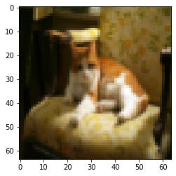
# 加载数据
train_x_orig, train_y, test_x_orig, test_y, classes = load_data()
# Example of a picture
index = 7
plt.imshow(train_x_orig[index])
print ("y = " + str(train_y[0,index]) + ". It's a " + classes[train_y[0,index]].decode("utf-8") +  " picture.")

y = 1. It's a cat picture.

【HW】L1W4-深度神经网络 - 图34

# Explore your dataset 
m_train = train_x_orig.shape[0]
num_px = train_x_orig.shape[1]
m_test = test_x_orig.shape[0]
print ("Number of training examples: " + str(m_train))
print ("Number of testing examples: " + str(m_test))
print ("Each image is of size: (" + str(num_px) + ", " + str(num_px) + ", 3)")
print ("train_x_orig shape: " + str(train_x_orig.shape))
print ("train_y shape: " + str(train_y.shape))
print ("test_x_orig shape: " + str(test_x_orig.shape))
print ("test_y shape: " + str(test_y.shape))

Number of training examples: 209
Number of testing examples: 50
Each image is of size: (64, 64, 3)
train_x_orig shape: (209, 64, 64, 3)
train_y shape: (1, 209)
test_x_orig shape: (50, 64, 64, 3)
test_y shape: (1, 50)

与往常一样，在将图像输入到网络之前，需要对图像进行重塑和标准化。下面单元格给出了相关代码。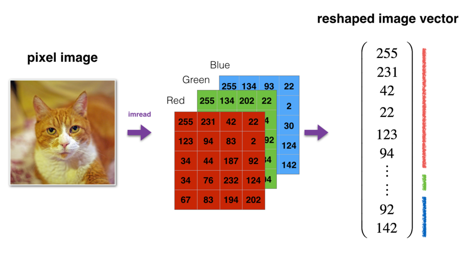

图：图像转换为向量。

# Reshape the training and test examples 
train_x_flatten = train_x_orig.reshape(train_x_orig.shape[0], -1).T   # The "-1" makes reshape flatten the remaining dimensions
test_x_flatten = test_x_orig.reshape(test_x_orig.shape[0], -1).T
# Standardize data to have feature values between 0 and 1.
train_x = train_x_flatten/255.
test_x = test_x_flatten/255.
print ("train_x's shape: " + str(train_x.shape))
print ("test_x's shape: " + str(test_x.shape))

train_x's shape: (12288, 209)
test_x's shape: (12288, 50)

现在你已经熟悉了数据集，是时候建立一个深度神经网络来区分猫图像和非猫图像了。

你将建立两个不同的模型：

2层神经网络
L层深度神经网络
然后，你将比较这些模型的性能，并尝试不同的值。

通用步骤
与往常一样，你将遵循深度学习步骤来构建模型：

初始化参数/定义超参数
循环num_iterations次：
a. 正向传播
b. 计算损失函数
C. 反向传播
d. 更新参数（使用参数和反向传播的梯度）
使用训练好的参数来预测标签

现在让我们实现这两个模型！

2层的神经网络

### CONSTANTS DEFINING THE MODEL ####
n_x = 12288     # num_px * num_px * 3
n_h = 7
n_y = 1
layers_dims = (n_x, n_h, n_y)

# GRADED FUNCTION: two_layer_model
def two_layer_model(X, Y, layers_dims, learning_rate = 0.0075, num_iterations = 3000, print_cost=False):
    """
    Implements a two-layer neural network: LINEAR->RELU->LINEAR->SIGMOID.
    Returns:
    parameters -- a dictionary containing W1, W2, b1, and b2
    """
    np.random.seed(1)
    grads = {}
    costs = []                              # to keep track of the cost
    m = X.shape[1]                           # number of examples
    (n_x, n_h, n_y) = layers_dims
    # Initialize parameters dictionary, by calling one of the functions you'd previously implemented
    ### START CODE HERE ### (≈ 1 line of code)
    parameters = initialize_parameters(n_x, n_h, n_y)
    ### END CODE HERE ###
    # Get W1, b1, W2 and b2 from the dictionary parameters.
    W1 = parameters["W1"]
    b1 = parameters["b1"]
    W2 = parameters["W2"]
    b2 = parameters["b2"]
    # Loop (gradient descent)
    for i in range(0, num_iterations):
        # Forward propagation: LINEAR -> RELU -> LINEAR -> SIGMOID. 
        A1, cache1 =linear_activation_forward(X, W1, b1, activation = "relu")
        A2, cache2 = linear_activation_forward(A1, W2, b2, activation = "sigmoid")
        # Compute cost
        cost = compute_cost(A2, Y)
        # Initializing backward propagation
        dA2 = - (np.divide(Y, A2) - np.divide(1 - Y, 1 - A2))
        # Backward propagation.
        dA1, dW2, db2 = linear_activation_backward(dA2, cache2, activation = "sigmoid")
        dA0, dW1, db1 = linear_activation_backward(dA1, cache1, activation = "relu")
        # Set grads['dWl'] to dW1, grads['db1'] to db1, grads['dW2'] to dW2, grads['db2'] to db2
        grads['dW1'] = dW1
        grads['db1'] = db1
        grads['dW2'] = dW2
        grads['db2'] = db2
        # Update parameters.
        parameters = update_parameters(parameters, grads, learning_rate)
        # Retrieve W1, b1, W2, b2 from parameters
        W1 = parameters["W1"]
        b1 = parameters["b1"]
        W2 = parameters["W2"]
        b2 = parameters["b2"]
        # Print the cost every 100 training example
        if print_cost and i % 100 == 0:
            print("Cost after iteration {}: {}".format(i, np.squeeze(cost)))
        if print_cost and i % 100 == 0:
            costs.append(cost)
    # plot the cost
    plt.plot(np.squeeze(costs))
    plt.ylabel('cost')
    plt.xlabel('iterations (per tens)')
    plt.title("Learning rate =" + str(learning_rate))
    plt.show()
    return parameters

parameters = two_layer_model(train_x, train_y, layers_dims = (n_x, n_h, n_y), num_iterations = 2500, print_cost=True)

Cost after iteration 0: 0.693049735659989
Cost after iteration 100: 0.6464320953428849
Cost after iteration 200: 0.6325140647912678
Cost after iteration 300: 0.6015024920354665
Cost after iteration 400: 0.5601966311605747
Cost after iteration 500: 0.5158304772764729
Cost after iteration 600: 0.4754901313943325
Cost after iteration 700: 0.43391631512257495
Cost after iteration 800: 0.4007977536203887
Cost after iteration 900: 0.35807050113237976
Cost after iteration 1000: 0.33942815383664127
Cost after iteration 1100: 0.30527536361962654
Cost after iteration 1200: 0.2749137728213016
Cost after iteration 1300: 0.24681768210614846
Cost after iteration 1400: 0.19850735037466097
Cost after iteration 1500: 0.17448318112556657
Cost after iteration 1600: 0.1708076297809689
Cost after iteration 1700: 0.11306524562164715
Cost after iteration 1800: 0.09629426845937145
Cost after iteration 1900: 0.08342617959726863
Cost after iteration 2000: 0.07439078704319078
Cost after iteration 2100: 0.06630748132267933
Cost after iteration 2200: 0.0591932950103817
Cost after iteration 2300: 0.05336140348560554
Cost after iteration 2400: 0.04855478562877016

【HW】L1W4-深度神经网络 - 图36

L层的神经网络

layers_dims = [12288, 20, 7, 5, 1] #  5-layer model
# GRADED FUNCTION: L_layer_model
def L_layer_model(X, Y, layers_dims, learning_rate = 0.0075, num_iterations = 3000, print_cost=False):#lr was 0.009
    np.random.seed(1)
    costs = []                         # keep track of cost
    # Parameters initialization.
    parameters = initialize_parameters_deep(layers_dims)
    # Loop (gradient descent)
    for i in range(0, num_iterations):
        # Forward propagation: [LINEAR -> RELU]*(L-1) -> LINEAR -> SIGMOID.
        AL, caches = L_model_forward(X, parameters)
        # Compute cost.
        cost = compute_cost(AL, Y)
        # Backward propagation.
        grads = L_model_backward(AL, Y, caches)
        # Update parameters.
        parameters = update_parameters(parameters, grads, learning_rate)
        # Print the cost every 100 training example
        if print_cost and i % 100 == 0:
            print ("Cost after iteration %i: %f" %(i, cost))
        if print_cost and i % 100 == 0:
            costs.append(cost)
    # plot the cost
    plt.plot(np.squeeze(costs))
    plt.ylabel('cost')
    plt.xlabel('iterations (per tens)')
    plt.title("Learning rate =" + str(learning_rate))
    plt.show()
    return parameters

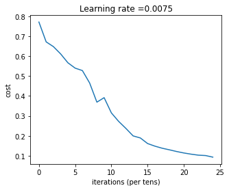
parameters = L_layer_model(train_x, train_y, layers_dims, num_iterations = 2500, print_cost = True)

Cost after iteration 0: 0.771749
Cost after iteration 100: 0.672053
Cost after iteration 200: 0.648263
Cost after iteration 300: 0.611507
Cost after iteration 400: 0.567047
Cost after iteration 500: 0.540138
Cost after iteration 600: 0.527930
Cost after iteration 700: 0.465477
Cost after iteration 800: 0.369126
Cost after iteration 900: 0.391747
Cost after iteration 1000: 0.315187
Cost after iteration 1100: 0.272700
Cost after iteration 1200: 0.237419
Cost after iteration 1300: 0.199601
Cost after iteration 1400: 0.189263
Cost after iteration 1500: 0.161189
Cost after iteration 1600: 0.148214
Cost after iteration 1700: 0.137775
Cost after iteration 1800: 0.129740
Cost after iteration 1900: 0.121225
Cost after iteration 2000: 0.113821
Cost after iteration 2100: 0.107839
Cost after iteration 2200: 0.102855
Cost after iteration 2300: 0.100897
Cost after iteration 2400: 0.092878

【HW】L1W4-深度神经网络 - 图37

查看训练和测试集的预测结果

def predict(X, y, parameters):
    m = X.shape[1]
    n = len(parameters) // 2 # number of layers in the neural network
    p = np.zeros((1,m))
    # Forward propagation
    probas, caches = L_model_forward(X, parameters)
    # convert probas to 0/1 predictions
    for i in range(0, probas.shape[1]):
        if probas[0,i] > 0.5:
            p[0,i] = 1
        else:
            p[0,i] = 0
    #print results
    #print ("predictions: " + str(p))
    #print ("true labels: " + str(y))
    print("Accuracy: "  + str(np.sum((p == y)/m)))
    return p

pred_train = predict(train_x, train_y, parameters)

Accuracy: 0.9856459330143539

pred_test = predict(test_x, test_y, parameters)

Accuracy: 0.8

结果分析

首先，让我们看一下L层模型标记错误的一些图像。这将显示一些分类错误的图像。

def print_mislabeled_images(classes, X, y, p):
    """
    Plots images where predictions and truth were different.
    X -- dataset
    y -- true labels
    p -- predictions
    """
    a = p + y
    mislabeled_indices = np.asarray(np.where(a == 1))
    plt.rcParams['figure.figsize'] = (40.0, 40.0) # set default size of plots
    num_images = len(mislabeled_indices[0])
    for i in range(num_images):
        index = mislabeled_indices[1][i]
        plt.subplot(2, num_images, i + 1)
        plt.imshow(X[:,index].reshape(64,64,3), interpolation='nearest')
        plt.axis('off')
        plt.title("Prediction: " + classes[int(p[0,index])].decode("utf-8") + " \n Class: " + classes[y[0,index]].decode("utf-8"))

print_mislabeled_images(classes, test_x, test_y, pred_test)

【HW】L1W4-深度神经网络 - 图38

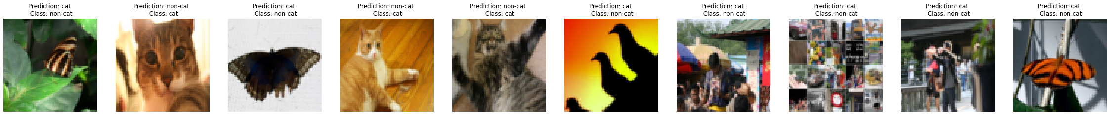
该模型在表现效果较差的的图像包括：

猫身处于异常位置
图片背景与猫颜色类似
猫的种类和颜色稀有
相机角度
图片的亮度
比例变化（猫的图像很大或很小）

【HW】L1W4-深度神经网络