初始化
欢迎来到“改善深度神经网络”的第一项作业。
训练神经网络需要指定权重的初始值,而一个好的初始化方法将有助于网络学习。不同的初始化导致的不同结果。好的初始化可以:
- 加快梯度下降、模型收敛
- 减小梯度下降收敛过程中训练(和泛化)出现误差的几率
首先,运行以下单元格以加载包和用于分类的二维数据集。
import numpy as npimport matplotlib.pyplot as pltimport sklearnimport sklearn.datasetsfrom init_utils import sigmoid, relu, compute_loss, forward_propagation, backward_propagationfrom init_utils import update_parameters, predict, load_dataset, plot_decision_boundary, predict_dec%matplotlib inlineplt.rcParams['figure.figsize'] = (7.0, 4.0) # set default size of plotsplt.rcParams['image.interpolation'] = 'nearest'plt.rcParams['image.cmap'] = 'gray'# load image dataset: blue/red dots in circlestrain_X, train_Y, test_X, test_Y = load_dataset()
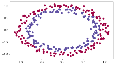
我们希望分类器将蓝点和红点分开。
1 神经网络模型
你将使用已经实现了的3层神经网络。 下面是你将尝试的初始化方法:
- 零初始化 :在输入参数中设置
initialization = "zeros"。 - 随机初始化 :在输入参数中设置
initialization = "random",这会将权重初始化为较大的随机值。 - He初始化 :在输入参数中设置
initialization = "he",这会根据He等人(2015)的论文将权重初始化为按比例缩放的随机值。
说明:请快速阅读并运行以下代码,在下一部分中,你将实现此model()调用的三种初始化方法。
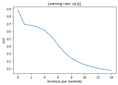
def model(X, Y, learning_rate = 0.01, num_iterations = 15000, print_cost = True, initialization = "he"):"""Implements a three-layer neural network: LINEAR->RELU->LINEAR->RELU->LINEAR->SIGMOID.Arguments:X -- input data, of shape (2, number of examples)Y -- true "label" vector (containing 0 for red dots; 1 for blue dots), of shape (1, number of examples)initialization -- flag to choose which initialization to use ("zeros","random" or "he")Returns:parameters -- parameters learnt by the model"""grads = {}costs = [] # to keep track of the lossm = X.shape[1] # number of exampleslayers_dims = [X.shape[0], 10, 5, 1]# Initialize parameters dictionary.if initialization == "zeros":parameters = initialize_parameters_zeros(layers_dims)elif initialization == "random":parameters = initialize_parameters_random(layers_dims)elif initialization == "he":parameters = initialize_parameters_he(layers_dims)# Loop (gradient descent)for i in range(0, num_iterations):# Forward propagation: LINEAR -> RELU -> LINEAR -> RELU -> LINEAR -> SIGMOID.a3, cache = forward_propagation(X, parameters)# Losscost = compute_loss(a3, Y)# Backward propagation.grads = backward_propagation(X, Y, cache)# Update parameters.parameters = update_parameters(parameters, grads, learning_rate)# Print the loss every 1000 iterationsif print_cost and i % 1000 == 0:print("Cost after iteration {}: {}".format(i, cost))costs.append(cost)# plot the lossplt.plot(costs)plt.ylabel('cost')plt.xlabel('iterations (per hundreds)')plt.title("Learning rate =" + str(learning_rate))plt.show()return parameters
2 零初始化
在神经网络中有两种类型的参数要初始化:
- 权重矩阵
#card=math&code=%28W%5E%7B%5B1%5D%7D%2C%20W%5E%7B%5B2%5D%7D%2C%20W%5E%7B%5B3%5D%7D%2C%20…%2C%20W%5E%7B%5BL-1%5D%7D%2C%20W%5E%7B%5BL%5D%7D%29&id=iO2xL)
- 偏差向量
#card=math&code=%28b%5E%7B%5B1%5D%7D%2C%20b%5E%7B%5B2%5D%7D%2C%20b%5E%7B%5B3%5D%7D%2C%20…%2C%20b%5E%7B%5BL-1%5D%7D%2C%20b%5E%7B%5BL%5D%7D%29&id=GezSB)
练习:实现以下函数以将所有参数初始化为零。 稍后你会看到此方法会报错,因为它无法“打破对称性”。
# GRADED FUNCTION: initialize_parameters_zerosdef initialize_parameters_zeros(layers_dims):parameters = {}L = len(layers_dims) # number of layers in the networkfor l in range(1, L):### START CODE HERE ### (≈ 2 lines of code)parameters['W' + str(l)] = np.zeros((layers_dims[l],layers_dims[l-1]))parameters['b' + str(l)] = np.zeros((layers_dims[l],1))### END CODE HERE ###return parameters
parameters = initialize_parameters_zeros([3,2,1])print("W1 = " + str(parameters["W1"]))print("b1 = " + str(parameters["b1"]))print("W2 = " + str(parameters["W2"]))print("b2 = " + str(parameters["b2"]))
W1 = [[0. 0. 0.][0. 0. 0.]]b1 = [[0.][0.]]W2 = [[0. 0.]]b2 = [[0.]]
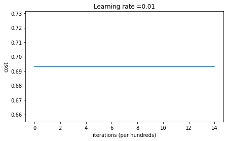
运行以下代码使用零初始化并迭代15,000次以训练模型。
parameters = model(train_X, train_Y, initialization = "zeros")print ("On the train set:")predictions_train = predict(train_X, train_Y, parameters)print ("On the test set:")predictions_test = predict(test_X, test_Y, parameters)
Cost after iteration 0: 0.6931471805599453Cost after iteration 1000: 0.6931471805599453Cost after iteration 2000: 0.6931471805599453Cost after iteration 3000: 0.6931471805599453Cost after iteration 4000: 0.6931471805599453Cost after iteration 5000: 0.6931471805599453Cost after iteration 6000: 0.6931471805599453Cost after iteration 7000: 0.6931471805599453Cost after iteration 8000: 0.6931471805599453Cost after iteration 9000: 0.6931471805599453Cost after iteration 10000: 0.6931471805599455Cost after iteration 11000: 0.6931471805599453Cost after iteration 12000: 0.6931471805599453Cost after iteration 13000: 0.6931471805599453Cost after iteration 14000: 0.6931471805599453
On the train set:Accuracy: 0.5On the test set:Accuracy: 0.5
性能确实很差,损失也没有真正降低,该算法的性能甚至不如随机猜测。为什么呢?让我们看一下预测的详细信息和决策边界:
print ("predictions_train = " + str(predictions_train))print ("predictions_test = " + str(predictions_test))
predictions_train = [[0 0 0 0 0 0 0 0 0 0 0 0 0 0 0 0 0 0 0 0 0 0 0 0 0 0 0 0 0 0 0 0 0 0 0 00 0 0 0 0 0 0 0 0 0 0 0 0 0 0 0 0 0 0 0 0 0 0 0 0 0 0 0 0 0 0 0 0 0 0 00 0 0 0 0 0 0 0 0 0 0 0 0 0 0 0 0 0 0 0 0 0 0 0 0 0 0 0 0 0 0 0 0 0 0 00 0 0 0 0 0 0 0 0 0 0 0 0 0 0 0 0 0 0 0 0 0 0 0 0 0 0 0 0 0 0 0 0 0 0 00 0 0 0 0 0 0 0 0 0 0 0 0 0 0 0 0 0 0 0 0 0 0 0 0 0 0 0 0 0 0 0 0 0 0 00 0 0 0 0 0 0 0 0 0 0 0 0 0 0 0 0 0 0 0 0 0 0 0 0 0 0 0 0 0 0 0 0 0 0 00 0 0 0 0 0 0 0 0 0 0 0 0 0 0 0 0 0 0 0 0 0 0 0 0 0 0 0 0 0 0 0 0 0 0 00 0 0 0 0 0 0 0 0 0 0 0 0 0 0 0 0 0 0 0 0 0 0 0 0 0 0 0 0 0 0 0 0 0 0 00 0 0 0 0 0 0 0 0 0 0 0]]predictions_test = [[0 0 0 0 0 0 0 0 0 0 0 0 0 0 0 0 0 0 0 0 0 0 0 0 0 0 0 0 0 0 0 0 0 0 0 00 0 0 0 0 0 0 0 0 0 0 0 0 0 0 0 0 0 0 0 0 0 0 0 0 0 0 0 0 0 0 0 0 0 0 00 0 0 0 0 0 0 0 0 0 0 0 0 0 0 0 0 0 0 0 0 0 0 0 0 0 0 0]]
plt.title("Model with Zeros initialization")axes = plt.gca()axes.set_xlim([-1.5,1.5])axes.set_ylim([-1.5,1.5])plot_decision_boundary(lambda x: predict_dec(parameters, x.T), train_X, train_Y)
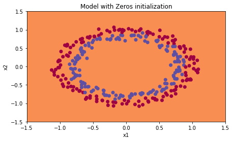
该模型预测的每个示例都为0。
通常,将所有权重初始化为零会导致网络无法打破对称性。 这意味着每一层中的每个神经元都将学习相同的东西,并且你不妨训练每一层的神经网络,该网络的性能不如线性分类器,例如逻辑回归。
总结:
- 权重
应该随机初始化以打破对称性。
- 将偏差
初始化为零是可以的。只要随机初始化了
,对称性就会被破坏。
3 随机初始化
为了打破对称性,让我们随机设置权重。 在随机初始化之后,每个神经元可以继续学习其输入的不同特征。
练习:实现以下函数,将权重初始化为较大的随机值(按10缩放),并将偏差设为0。 将 `np.random.randn(..,..) 10用于权重,将np.zeros((.., ..))用于偏差。我们使用固定的np.random.seed(..)`,以确保你的“随机”权重与我们的权重匹配。因此,如果运行几次代码后参数初始值始终相同,也请不要疑惑。
# GRADED FUNCTION: initialize_parameters_randomdef initialize_parameters_random(layers_dims):np.random.seed(3) # This seed makes sure your "random" numbers will be the as oursparameters = {}L = len(layers_dims) # integer representing the number of layersfor l in range(1, L):### START CODE HERE ### (≈ 2 lines of code)parameters['W' + str(l)] = np.random.randn(layers_dims[l],layers_dims[l-1])*10parameters['b' + str(l)] = np.zeros((layers_dims[l],1))### END CODE HERE ###return parameters
parameters = initialize_parameters_random([3, 2, 1])print("W1 = " + str(parameters["W1"]))print("b1 = " + str(parameters["b1"]))print("W2 = " + str(parameters["W2"]))print("b2 = " + str(parameters["b2"]))
W1 = [[ 17.88628473 4.36509851 0.96497468][-18.63492703 -2.77388203 -3.54758979]]b1 = [[0.][0.]]W2 = [[-0.82741481 -6.27000677]]b2 = [[0.]]
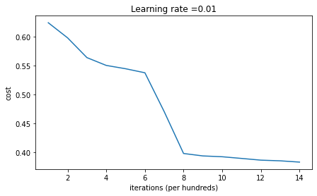
运行以下代码使用随机初始化迭代15,000次以训练模型。
parameters = model(train_X, train_Y, initialization = "random")print ("On the train set:")predictions_train = predict(train_X, train_Y, parameters)print ("On the test set:")predictions_test = predict(test_X, test_Y, parameters)
Cost after iteration 0: infCost after iteration 1000: 0.6239567039908781Cost after iteration 2000: 0.5978043872838292Cost after iteration 3000: 0.563595830364618Cost after iteration 4000: 0.5500816882570866Cost after iteration 5000: 0.5443417928662615Cost after iteration 6000: 0.5373553777823036Cost after iteration 7000: 0.4700141958024487Cost after iteration 8000: 0.3976617665785177Cost after iteration 9000: 0.39344405717719166Cost after iteration 10000: 0.39201765232720626Cost after iteration 11000: 0.38910685278803786Cost after iteration 12000: 0.38612995897697244Cost after iteration 13000: 0.3849735792031832Cost after iteration 14000: 0.38275100578285265
On the train set:Accuracy: 0.83On the test set:Accuracy: 0.86
因为数值舍入,你可能在0迭代之后看到损失为”inf”,我们会在之后用更复杂的数字实现解决此问题。
总之,看起来你的对称性已打破,这会带来更好的结果。 相比之前,模型不再输出全0的结果了。
print (predictions_train)print (predictions_test)
[[1 0 1 1 0 0 1 1 1 1 1 0 1 0 0 1 0 1 1 0 0 0 1 0 1 1 1 1 1 1 0 1 1 0 0 11 1 1 1 1 1 1 0 1 1 1 1 0 1 0 1 1 1 1 0 0 1 1 1 1 0 1 1 0 1 0 1 1 1 1 00 0 0 0 1 0 1 0 1 1 1 0 0 1 1 1 1 1 1 0 0 1 1 1 0 1 1 0 1 0 1 1 0 1 1 01 0 1 1 0 0 1 0 0 1 1 0 1 1 1 0 1 0 0 1 0 1 1 1 1 1 1 1 0 1 1 0 0 1 1 00 0 1 0 1 0 1 0 1 1 1 0 0 1 1 1 1 0 1 1 0 1 0 1 1 0 1 0 1 1 1 1 0 1 1 11 0 1 0 1 0 1 1 1 1 0 1 1 0 1 1 0 1 1 0 1 0 1 1 1 0 1 1 1 0 1 0 1 0 0 10 1 1 0 1 1 0 1 1 0 1 1 1 0 1 1 1 1 0 1 0 0 1 1 0 1 1 1 0 0 0 1 1 0 1 11 1 0 1 1 0 1 1 1 0 0 1 0 0 0 1 0 0 0 1 1 1 1 0 0 0 0 1 1 1 1 0 0 1 1 11 1 1 1 0 0 0 1 1 1 1 0]][[1 1 1 1 0 1 0 1 1 0 1 1 1 0 0 0 0 1 0 1 0 0 1 0 1 0 1 1 1 1 1 0 0 0 0 10 1 1 0 0 1 1 1 1 1 0 1 1 1 0 1 0 1 1 0 1 0 1 0 1 1 1 1 1 1 1 1 1 0 1 01 1 1 1 1 0 1 0 0 1 0 0 0 1 1 0 1 1 0 0 0 1 1 0 1 1 0 0]]
plt.title("Model with large random initialization")axes = plt.gca()axes.set_xlim([-1.5,1.5])axes.set_ylim([-1.5,1.5])plot_decision_boundary(lambda x: predict_dec(parameters, x.T), train_X, train_Y)
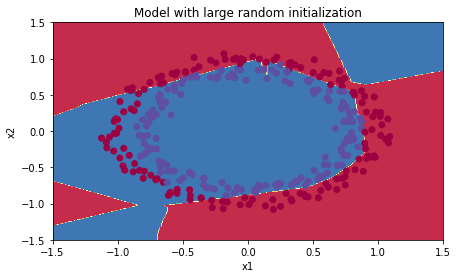
观察:
- 损失一开始很高是因为较大的随机权重值,对于某些数据,最后一层激活函数sigmoid输出的结果非常接近0或1,并且当该示例数据预测错误时,将导致非常高的损失。当
%20%3D%20%5Clog(0)#card=math&code=%5Clog%28a%5E%7B%5B3%5D%7D%29%20%3D%20%5Clog%280%29&id=OU83o)时,损失达到无穷大。
- 初始化不当会导致梯度消失/爆炸,同时也会减慢优化算法的速度。
- 训练较长时间的网络,将会看到更好的结果,但是使用太大的随机数进行初始化会降低优化速度。
总结:
- 将权重初始化为非常大的随机值效果不佳。
- 初始化为较小的随机值会更好。重要的问题是:这些随机值应为多小?让我们在下一部分中找到答案!
4 He初始化
最后,让我们尝试一下“He 初始化”,该名称以He等人的名字命名(类似于“Xavier初始化”,但Xavier初始化使用比例因子 sqrt(1./layers_dims[l-1])来表示权重 ,而He初始化使用
sqrt(2./layers_dims[l-1]))。
- Xavier初始化:
- normalized initialization:
- 假设激活函数关于0对称,且主要针对于全连接神经网络。适用于tanh和soft sign
- 论文地址:Understanding the difficulty of training deep feedforward neural networks
- 参考资料:
深度学习之参数初始化(一)——Xavier初始化
- He初始化:
- 适用于ReLU的初始化方法:
- 适用于Leaky ReLU的初始化方法:
其中,分别表示卷积层中卷积核的高和宽,
是当前层卷积核的个数。
- 论文地址:Delving Deep into Rectifiers: Surpassing Human-Level Performance on ImageNet Classification
- 参考资料:
深度学习之参数初始化(二)——Kaiming初始化
He初始化论文阅读笔记与实现


练习:实现以下函数,以He初始化来初始化参数。
提示:此函数类似于先前的initialize_parameters_random(...)。 唯一的不同是,无需将np.random.randn(..,..)乘以10,而是将其乘以,这是He初始化建议使用的ReLU激活层。
# GRADED FUNCTION: initialize_parameters_hedef initialize_parameters_he(layers_dims):np.random.seed(3)parameters = {}L = len(layers_dims) - 1 # integer representing the number of layersfor l in range(1, L + 1):### START CODE HERE ### (≈ 2 lines of code)parameters['W' + str(l)] = np.random.randn(layers_dims[l],layers_dims[l-1])*np.sqrt(2./layers_dims[l-1])parameters['b' + str(l)] = np.zeros((layers_dims[l],1))### END CODE HERE ###return parameters
parameters = initialize_parameters_he([2, 4, 1])
W1 = [[ 1.78862847 0.43650985][ 0.09649747 -1.8634927 ][-0.2773882 -0.35475898][-0.08274148 -0.62700068]]b1 = [[0.][0.][0.][0.]]W2 = [[-0.03098412 -0.33744411 -0.92904268 0.62552248]]b2 = [[0.]]
运行以下代码,使用He初始化并迭代15,000次以训练你的模型。
parameters = model(train_X, train_Y, initialization = "he")print ("On the train set:")predictions_train = predict(train_X, train_Y, parameters)print ("On the test set:")predictions_test = predict(test_X, test_Y, parameters)
Cost after iteration 0: 0.8830537463419761Cost after iteration 1000: 0.6879825919728063Cost after iteration 2000: 0.6751286264523371Cost after iteration 3000: 0.6526117768893805Cost after iteration 4000: 0.6082958970572938Cost after iteration 5000: 0.5304944491717495Cost after iteration 6000: 0.4138645817071794Cost after iteration 7000: 0.3117803464844441Cost after iteration 8000: 0.23696215330322562Cost after iteration 9000: 0.1859728720920684Cost after iteration 10000: 0.15015556280371808Cost after iteration 11000: 0.12325079292273551Cost after iteration 12000: 0.09917746546525937Cost after iteration 13000: 0.08457055954024283Cost after iteration 14000: 0.07357895962677366
On the train set:Accuracy: 0.9933333333333333On the test set:Accuracy: 0.96
plt.title("Model with He initialization")axes = plt.gca()axes.set_xlim([-1.5,1.5])axes.set_ylim([-1.5,1.5])plot_decision_boundary(lambda x: predict_dec(parameters, x.T), train_X, train_Y)
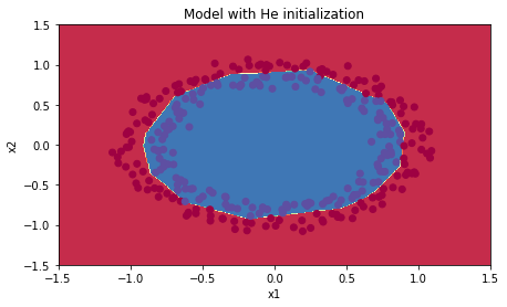
观察:
- 使用He初始化的模型可以在少量迭代中很好地分离蓝色点和红色点。
5 总结
我们已经学习了三种不同类型的初始化方法。对于相同的迭代次数和超参数,三种结果比较为:
| Model | 测试准确率 | 评价 |
|---|---|---|
| 零初始化的3层NN | 50% | 未能打破对称性 |
| 随机初始化的3层NN | 83% | 权重太大 |
| He初始化的3层NN | 99% | 推荐方法 |
此作业中应记住的内容:
欢迎来到本周的第二次作业。
深度学习模型具有很高的灵活性和能力,如果训练数据集不够大,将会造成一个严重的问题—过拟合。尽管它在训练集上效果很好,但是学到的网络不能应用到测试集中!
你将学习: 在深度学习模型中使用正则化。
首先导入要使用的包。
# import packagesimport numpy as npimport matplotlib.pyplot as pltfrom reg_utils import sigmoid, relu, plot_decision_boundary, initialize_parameters, load_2D_dataset, predict_decfrom reg_utils import compute_cost, predict, forward_propagation, backward_propagation, update_parametersimport sklearnimport sklearn.datasetsimport scipy.iofrom testCases import *%matplotlib inlineplt.rcParams['figure.figsize'] = (7.0, 4.0) # set default size of plotsplt.rcParams['image.interpolation'] = 'nearest'plt.rcParams['image.cmap'] = 'gray'
加载二维数据集如下。
train_X, train_Y, test_X, test_Y = load_2D_dataset()
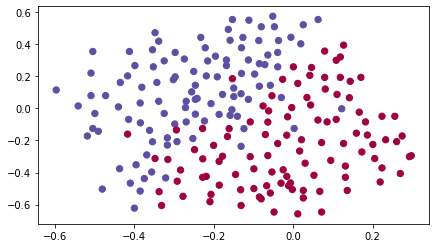
数据集分析:该数据集含有噪声,但看起来一条将左上半部分(蓝色)与右下半部分(红色)分开的对角线会很比较有效。
你将首先尝试非正则化模型。然后学习如何对其进行正则化,并决定选择哪种模型。
1 非正则化模型
首先,你将尝试不进行任何正则化的模型。然后,你将实现:
- L2 正则化 函数:
compute_cost_with_regularization()和backward_propagation_with_regularization() - Dropout 函数:
forward_propagation_with_dropout()和backward_propagation_with_dropout()
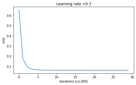
def model(X, Y, learning_rate = 0.3, num_iterations = 30000, print_cost = True, lambd = 0, keep_prob = 1):"""Implements a three-layer neural network: LINEAR->RELU->LINEAR->RELU->LINEAR->SIGMOID.Arguments:X -- input data, of shape (input size, number of examples)Y -- true "label" vector (1 for blue dot / 0 for red dot), of shape (output size, number of examples)lambd -- regularization hyperparameter, scalarkeep_prob - probability of keeping a neuron active during drop-out, scalar.Returns:parameters -- parameters learned by the model. They can then be used to predict."""grads = {}costs = [] # to keep track of the costm = X.shape[1] # number of exampleslayers_dims = [X.shape[0], 20, 3, 1]# Initialize parameters dictionary.parameters = initialize_parameters(layers_dims)# Loop (gradient descent)for i in range(0, num_iterations):# Forward propagation: LINEAR -> RELU -> LINEAR -> RELU -> LINEAR -> SIGMOID.if keep_prob == 1:a3, cache = forward_propagation(X, parameters)elif keep_prob < 1:a3, cache = forward_propagation_with_dropout(X, parameters, keep_prob)# Cost functionif lambd == 0:cost = compute_cost(a3, Y)else:cost = compute_cost_with_regularization(a3, Y, parameters, lambd)# Backward propagation.assert(lambd==0 or keep_prob==1) # it is possible to use both L2 regularization and dropout,# but this assignment will only explore one at a timeif lambd == 0 and keep_prob == 1:grads = backward_propagation(X, Y, cache)elif lambd != 0:grads = backward_propagation_with_regularization(X, Y, cache, lambd)elif keep_prob < 1:grads = backward_propagation_with_dropout(X, Y, cache, keep_prob)# Update parameters.parameters = update_parameters(parameters, grads, learning_rate)# Print the loss every 10000 iterationsif print_cost and i % 10000 == 0:print("Cost after iteration {}: {}".format(i, cost))if print_cost and i % 1000 == 0:costs.append(cost)# plot the costplt.plot(costs)plt.ylabel('cost')plt.xlabel('iterations (x1,000)')plt.title("Learning rate =" + str(learning_rate))plt.show()return parameters
让我们在不进行任何正则化的情况下训练模型,并观察训练/测试集的准确性。
parameters = model(train_X, train_Y)print ("On the training set:")predictions_train = predict(train_X, train_Y, parameters)print ("On the test set:")predictions_test = predict(test_X, test_Y, parameters)
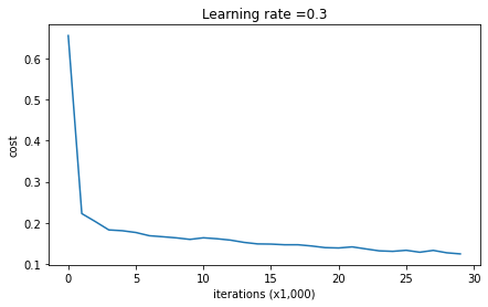
On the training set:Accuracy: 0.9478672985781991On the test set:Accuracy: 0.915
训练精度为94.8%,而测试精度为91.5%。这是基准模型的表现(你将观察到正则化对该模型的影响)。运行以下代码以绘制模型的决策边界。
plt.title("Model without regularization")axes = plt.gca()axes.set_xlim([-0.75,0.40])axes.set_ylim([-0.75,0.65])plot_decision_boundary(lambda x: predict_dec(parameters, x.T), train_X, train_Y)
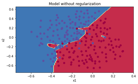
非正则化模型显然过度拟合了训练集,拟合了一些噪声点!现在让我们看一下减少过拟合的两种手段。
2 L2正则化
2.1 带有L2正则的正向传播
避免过拟合的标准方法称为 L2正则化,它将损失函数从:
%7D%5Clog%5Cleft(a%5E%7B%5BL%5D(i)%7D%5Cright)%20%2B%20(1-y%5E%7B(i)%7D)%5Clog%5Cleft(1-%20a%5E%7B%5BL%5D(i)%7D%5Cright)%20%5Clarge%7B)%7D%20%5Ctag%7B1%7D%0A#card=math&code=J%20%3D%20-%5Cfrac%7B1%7D%7Bm%7D%20%5Csum%5Climits_%7Bi%20%3D%201%7D%5E%7Bm%7D%20%5Clarge%7B%28%7D%5Csmall%20%20y%5E%7B%28i%29%7D%5Clog%5Cleft%28a%5E%7B%5BL%5D%28i%29%7D%5Cright%29%20%2B%20%281-y%5E%7B%28i%29%7D%29%5Clog%5Cleft%281-%20a%5E%7B%5BL%5D%28i%29%7D%5Cright%29%20%5Clarge%7B%29%7D%20%5Ctag%7B1%7D%0A&id=JUHFb)
修改到:
%7D%5Clog%5Cleft(a%5E%7B%5BL%5D(i)%7D%5Cright)%20%2B%20(1-y%5E%7B(i)%7D)%5Clog%5Cleft(1-%20a%5E%7B%5BL%5D(i)%7D%5Cright)%20%5Clarge%7B)%7D%20%7D%5Ctext%7Bcross-entropy%20cost%7D%20%2B%20%5Cunderbrace%7B%5Cfrac%7B1%7D%7Bm%7D%20%5Cfrac%7B%5Clambda%7D%7B2%7D%20%5Csum%5Climits_l%5Csum%5Climits_k%5Csum%5Climits_j%20W%7Bk%2Cj%7D%5E%7B%5Bl%5D2%7D%20%7D%5Ctext%7BL2%20regularization%20cost%7D%20%5Ctag%7B2%7D%0A#card=math&code=J%7Bregularized%7D%20%3D%20%5Csmall%20%5Cunderbrace%7B-%5Cfrac%7B1%7D%7Bm%7D%20%5Csum%5Climits%7Bi%20%3D%201%7D%5E%7Bm%7D%20%5Clarge%7B%28%7D%5Csmall%20y%5E%7B%28i%29%7D%5Clog%5Cleft%28a%5E%7B%5BL%5D%28i%29%7D%5Cright%29%20%2B%20%281-y%5E%7B%28i%29%7D%29%5Clog%5Cleft%281-%20a%5E%7B%5BL%5D%28i%29%7D%5Cright%29%20%5Clarge%7B%29%7D%20%7D%5Ctext%7Bcross-entropy%20cost%7D%20%2B%20%5Cunderbrace%7B%5Cfrac%7B1%7D%7Bm%7D%20%5Cfrac%7B%5Clambda%7D%7B2%7D%20%5Csum%5Climitsl%5Csum%5Climits_k%5Csum%5Climits_j%20W%7Bk%2Cj%7D%5E%7B%5Bl%5D2%7D%20%7D_%5Ctext%7BL2%20regularization%20cost%7D%20%5Ctag%7B2%7D%0A&id=wBGvi)
让我们修改损失并观察结果。
练习:实现compute_cost_with_regularization(),以计算公式(2)的损失。要计算 ,请使用:
np.sum(np.square(Wl))
请注意,你必须对,
和
执行此操作,然后将三个项相加并乘以
。
# GRADED FUNCTION: compute_cost_with_regularizationdef compute_cost_with_regularization(A3, Y, parameters, lambd):"""Implement the cost function with L2 regularization. See formula (2) above.Arguments:A3 -- post-activation, output of forward propagation, of shape (output size, number of examples)Y -- "true" labels vector, of shape (output size, number of examples)parameters -- python dictionary containing parameters of the modelReturns:cost - value of the regularized loss function (formula (2))"""m = Y.shape[1]W1 = parameters["W1"]W2 = parameters["W2"]W3 = parameters["W3"]cross_entropy_cost = compute_cost(A3, Y) # This gives you the cross-entropy part of the cost### START CODE HERE ### (approx. 1 line)L2_regularization_cost = 1./m * lambd/2 * (np.sum(W1**2) + np.sum(W2**2) + np.sum(W3**2))### END CODER HERE ###cost = cross_entropy_cost + L2_regularization_costreturn cost
A3, Y_assess, parameters = compute_cost_with_regularization_test_case()print("cost = " + str(compute_cost_with_regularization(A3, Y_assess, parameters, lambd = 0.1)))
预期输出:
cost = 1.7864859451590758
2.2 带有L2正则的反向传播
当然,因为你更改了损失,所以还必须更改反向传播! 必须针对新损失函数计算所有梯度。
练习:实现正则化后的反向传播。更改仅涉及dW1,dW2和dW3。对于每一个,你必须添加正则化项的梯度(%20%3D%20%5Cfrac%7B%5Clambda%7D%7Bm%7D%20W#card=math&code=%5Cfrac%7Bd%7D%7BdW%7D%20%28%20%5Cfrac%7B1%7D%7B2%7D%5Cfrac%7B%5Clambda%7D%7Bm%7D%20%20W%5E2%29%20%3D%20%5Cfrac%7B%5Clambda%7D%7Bm%7D%20W&id=TJeMi))。
# GRADED FUNCTION: backward_propagation_with_regularizationdef backward_propagation_with_regularization(X, Y, cache, lambd):"""Implements the backward propagation of our baseline model to which we added an L2 regularization.Arguments:X -- input dataset, of shape (input size, number of examples)Y -- "true" labels vector, of shape (output size, number of examples)cache -- cache output from forward_propagation()lambd -- regularization hyperparameter, scalarReturns:gradients -- A dictionary with the gradients with respect to each parameter, activation and pre-activation variables"""m = X.shape[1](Z1, A1, W1, b1, Z2, A2, W2, b2, Z3, A3, W3, b3) = cachedZ3 = A3 - Y### START CODE HERE ### (approx. 1 line)dW3 = 1./m * np.dot(dZ3, A2.T) + lambd / m * W3### END CODE HERE ###db3 = 1./m * np.sum(dZ3, axis=1, keepdims = True)dA2 = np.dot(W3.T, dZ3)dZ2 = np.multiply(dA2, np.int64(A2 > 0))### START CODE HERE ### (approx. 1 line)dW2 = 1./m * np.dot(dZ2, A1.T) + lambd / m * W2### END CODE HERE ###db2 = 1./m * np.sum(dZ2, axis=1, keepdims = True)dA1 = np.dot(W2.T, dZ2)dZ1 = np.multiply(dA1, np.int64(A1 > 0))### START CODE HERE ### (approx. 1 line)dW1 = 1./m * np.dot(dZ1, X.T) + lambd / m * W1### END CODE HERE ###db1 = 1./m * np.sum(dZ1, axis=1, keepdims = True)gradients = {"dZ3": dZ3, "dW3": dW3, "db3": db3,"dA2": dA2,"dZ2": dZ2, "dW2": dW2, "db2": db2, "dA1": dA1,"dZ1": dZ1, "dW1": dW1, "db1": db1}return gradients
X_assess, Y_assess, cache = backward_propagation_with_regularization_test_case()grads = backward_propagation_with_regularization(X_assess, Y_assess, cache, lambd = 0.7)print ("dW1 = "+ str(grads["dW1"]))print ("dW2 = "+ str(grads["dW2"]))print ("dW3 = "+ str(grads["dW3"]))
dW1 = [[-0.25604646 0.12298827 -0.28297129][-0.17706303 0.34536094 -0.4410571 ]]dW2 = [[ 0.79276486 0.85133918][-0.0957219 -0.01720463][-0.13100772 -0.03750433]]dW3 = [[-1.77691347 -0.11832879 -0.09397446]]
预期输出:
dW1 = [[-0.25604646 0.12298827 -0.28297129]
[-0.17706303 0.34536094 -0.4410571 ]]
dW2 = [[ 0.79276486 0.85133918]
[-0.0957219 -0.01720463]
[-0.13100772 -0.03750433]]
dW3 = [[-1.77691347 -0.11832879 -0.09397446]]
现在让我们使用L2正则化#card=math&code=%28%5Clambda%20%3D%200.7%29&id=rysY9)运行的模型。
model()函数将调用:
compute_cost_with_regularization代替compute_costbackward_propagation_with_regularization代替backward_propagation
parameters = model(train_X, train_Y, lambd = 0.7)print ("On the train set:")predictions_train = predict(train_X, train_Y, parameters)print ("On the test set:")predictions_test = predict(test_X, test_Y, parameters)
Cost after iteration 0: 0.6974484493131264Cost after iteration 10000: 0.26849188732822393Cost after iteration 20000: 0.2680916337127301
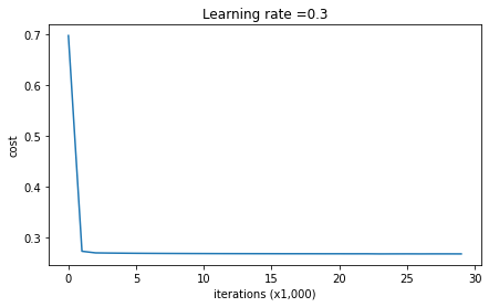
On the train set:Accuracy: 0.9383886255924171On the test set:Accuracy: 0.93
Nice!测试集的准确性提高到93%。你成功拯救了法国足球队!
模型不再过拟合训练数据了。让我们绘制决策边界看一下。
plt.title("Model with L2-regularization")axes = plt.gca()axes.set_xlim([-0.75,0.40])axes.set_ylim([-0.75,0.65])plot_decision_boundary(lambda x: predict_dec(parameters, x.T), train_X, train_Y)
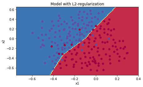
观察:
的值是你可以调整开发集的超参数。
- L2正则化使决策边界更平滑。如果
太大,则也可能“过度平滑”,从而使模型偏差较高。
L2正则化的原理:
L2正则化基于以下假设:权重较小的模型比权重较大的模型更简单。因此,通过对损失函数中权重的平方值进行惩罚,可以将所有权重驱动为较小的值。比重太大会使损失过高!这将导致模型更平滑,输出随着输入的变化而变化得更慢。
你应该记住 L2正则化的影响:
- 损失计算:
- 正则化条件会添加到损失函数中 - 反向传播函数:
- 有关权重矩阵的渐变中还有其他术语 - 权重最终变小(“权重衰减”):
- 权重被推到较小的值。
3 Dropout
最后,Dropout是广泛用于深度学习的正则化技术。
它会在每次迭代中随机关闭一些神经元。
要了解Dropout,可以思考这段对话:
- 朋友:“为什么你需要所有神经元来训练你的网络以分类图像?”。
- 你:“因为每个神经元都有权重,并且可以学习图像的特定特征/细节/形状。我拥有的神经元越多,模型学习的特征就越丰富!”
- 朋友:“我知道了,但是你确定你的神经元学习的是不同的特征而不是全部相同的特征吗?”
- 你:“这是个好问题……同一层中的神经元实际上并不关联。应该绝对有可能让他们学习相同的图像特征/形状/形式/细节…这是多余的。为此应该有一个解决方案。”
在每次迭代中,你以概率或以概率
(此处为50%)关闭此层的每个神经元。关闭的神经元对迭代的正向和反向传播均无助于训练。
图3:Dropout第一和第三隐藏层。层:我们平均关闭了40%的神经元。
层:我们平均关闭了20%的神经元。
当你关闭某些神经元时,实际上是在修改模型。通过Dropout,你的神经元对另一种特定神经元的激活变得不那么敏感,因为另一神经元可能随时关闭。
3.1 带有Dropout的正向传播
练习:实现带有Dropout的正向传播。你正在使用3层的神经网络,并将为第一和第二隐藏层添加Dropout。我们不会将Dropout应用于输入层或输出层。
说明:
关闭第一层和第二层中的某些神经元。为此,将执行4个步骤:
- 在讲座中,我们讨论了使用
np.random.rand()创建与形状相同的变量
的方法,以随机获取0到1之间的数。在这里,你将使用向量化的实现,创建一个与
的矩阵维度相同的随机矩阵$D^{[1]} = [d^{1} d^{1} … d^{1}] $。
- 通过对
中的值进行阈值设置,将
的每个条目设置为0(概率为
1-keep_prob)或1(概率为keep_prob)。提示:将矩阵X的所有条目设置为0(如果概率小于0.5)或1(如果概率大于0.5),则可以执行:X = (X < 0.5)。注意0和1分别对应False和True。 - 将
设置为
(关闭一些神经元)。你可以将
视为掩码,这样当它与另一个矩阵相乘时,关闭某些值。
- 将
除以
keep_prob。通过这样做,你可以确保损失结果仍具有与dropout相同的期望值。(此技术也称为反向dropout)
# GRADED FUNCTION: forward_propagation_with_dropoutdef forward_propagation_with_dropout(X, parameters, keep_prob = 0.5):"""Implements the forward propagation: LINEAR -> RELU + DROPOUT -> LINEAR -> RELU + DROPOUT -> LINEAR -> SIGMOID.Arguments:X -- input dataset, of shape (2, number of examples)parameters -- python dictionary containing your parameters "W1", "b1", "W2", "b2", "W3", "b3":W1 -- weight matrix of shape (20, 2)b1 -- bias vector of shape (20, 1)W2 -- weight matrix of shape (3, 20)b2 -- bias vector of shape (3, 1)W3 -- weight matrix of shape (1, 3)b3 -- bias vector of shape (1, 1)keep_prob - probability of keeping a neuron active during drop-out, scalarReturns:A3 -- last activation value, output of the forward propagation, of shape (1,1)cache -- tuple, information stored for computing the backward propagation"""np.random.seed(1)# retrieve parametersW1 = parameters["W1"]b1 = parameters["b1"]W2 = parameters["W2"]b2 = parameters["b2"]W3 = parameters["W3"]b3 = parameters["b3"]# LINEAR -> RELU -> LINEAR -> RELU -> LINEAR -> SIGMOIDZ1 = np.dot(W1, X) + b1A1 = relu(Z1)### START CODE HERE ### (approx. 4 lines) # Steps 1-4 below correspond to the Steps 1-4 described above.D1 = np.random.rand(len(A1), len(A1[0]))D1 = D1 < keep_probA1 = A1 * D1A1 = A1 / keep_prob### END CODE HERE ###Z2 = np.dot(W2, A1) + b2A2 = relu(Z2)### START CODE HERE ### (approx. 4 lines)D2 = np.random.rand(len(A2), len(A2[0]))D2 = D2 < keep_probA2 = A2 * D2A2 = A2 / keep_prob### END CODE HERE ###Z3 = np.dot(W3, A2) + b3A3 = sigmoid(Z3)cache = (Z1, D1, A1, W1, b1, Z2, D2, A2, W2, b2, Z3, A3, W3, b3)return A3, cache
X_assess, parameters = forward_propagation_with_dropout_test_case()A3, cache = forward_propagation_with_dropout(X_assess, parameters, keep_prob = 0.7)print ("A3 = " + str(A3))
A3 = [[0.36974721 0.00305176 0.04565099 0.49683389 0.36974721]]
预期输出:
A3 = [[0.36974721 0.00305176 0.04565099 0.49683389 0.36974721]]
3.2 带有dropout的反向传播
练习:实现带有dropout的反向传播。和之前一样,训练一个3层的网络。使用存储在缓存中的掩码和
,添加dropout到第一和第二个隐藏层。
说明:
带有dropout的反向传播实现上非常容易。你将必须执行2个步骤:
1.你先前通过在A1上应用掩码来关闭正向传播过程中的某些神经元。在反向传播中,你将必须将相同的掩码
重新应用于
dA1来关闭相同的神经元。
2.在正向传播过程中,你已将A1除以keep_prob。 因此,在反向传播中,必须再次将dA1除以keep_prob(计算的解释是,如果被
keep_prob缩放,则其派生的也由相同的
keep_prob缩放)。
# GRADED FUNCTION: backward_propagation_with_dropoutdef backward_propagation_with_dropout(X, Y, cache, keep_prob):"""Implements the backward propagation of our baseline model to which we added dropout.Arguments:X -- input dataset, of shape (2, number of examples)Y -- "true" labels vector, of shape (output size, number of examples)cache -- cache output from forward_propagation_with_dropout()keep_prob - probability of keeping a neuron active during drop-out, scalarReturns:gradients -- A dictionary with the gradients with respect to each parameter, activation and pre-activation variables"""m = X.shape[1](Z1, D1, A1, W1, b1, Z2, D2, A2, W2, b2, Z3, A3, W3, b3) = cachedZ3 = A3 - YdW3 = 1./m * np.dot(dZ3, A2.T)db3 = 1./m * np.sum(dZ3, axis=1, keepdims = True)dA2 = np.dot(W3.T, dZ3)### START CODE HERE ### (≈ 2 lines of code)dA2 = dA2 * D2dA2 = dA2 / keep_prob### END CODE HERE ###dZ2 = np.multiply(dA2, np.int64(A2 > 0))dW2 = 1./m * np.dot(dZ2, A1.T)db2 = 1./m * np.sum(dZ2, axis=1, keepdims = True)dA1 = np.dot(W2.T, dZ2)### START CODE HERE ### (≈ 2 lines of code)dA1 = dA1 * D1dA1 = dA1 / keep_prob### END CODE HERE ###dZ1 = np.multiply(dA1, np.int64(A1 > 0))dW1 = 1./m * np.dot(dZ1, X.T)db1 = 1./m * np.sum(dZ1, axis=1, keepdims = True)gradients = {"dZ3": dZ3, "dW3": dW3, "db3": db3,"dA2": dA2,"dZ2": dZ2, "dW2": dW2, "db2": db2, "dA1": dA1,"dZ1": dZ1, "dW1": dW1, "db1": db1}return gradients
X_assess, Y_assess, cache = backward_propagation_with_dropout_test_case()gradients = backward_propagation_with_dropout(X_assess, Y_assess, cache, keep_prob = 0.8)print ("dA1 = " + str(gradients["dA1"]))print ("dA2 = " + str(gradients["dA2"]))
输出:
dA1 = [[ 0.36544439 0. -0.00188233 0. -0.17408748]
[ 0.65515713 0. -0.00337459 0. -0. ]]
dA2 = [[ 0.58180856 0. -0.00299679 0. -0.27715731]
[ 0. 0.53159854 -0. 0.53159854 -0.34089673]
[ 0. 0. -0.00292733 0. -0. ]]
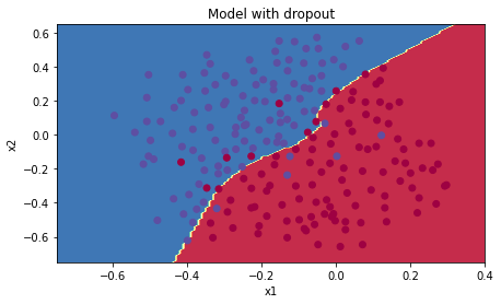
现在让我们使用dropout(keep_prob = 0.86)运行模型。 这意味着在每次迭代中,你都以24%的概率关闭第1层和第2层的每个神经元。
parameters = model(train_X, train_Y, keep_prob = 0.86, learning_rate = 0.3)print ("On the train set:")predictions_train = predict(train_X, train_Y, parameters)print ("On the test set:")predictions_test = predict(test_X, test_Y, parameters)
On the train set:Accuracy: 0.9289099526066351On the test set:Accuracy: 0.95
Dropout效果很好!测试精度再次提高(达到95%)!模型并未过拟合训练集,并且在测试集上表现很好。
运行以下代码以绘制决策边界。
plt.title("Model with dropout")axes = plt.gca()axes.set_xlim([-0.75,0.40])axes.set_ylim([-0.75,0.65])plot_decision_boundary(lambda x: predict_dec(parameters, x.T), train_X, train_Y)
注意:
- 使用dropout时的常见错误是在训练和测试中都使用。你只能在训练中使用dropout(随机删除节点)。
- 深度学习框架,例如tensorflow, PaddlePaddle, keras或者 caffe 附带dropout层的实现。不需强调-相信你很快就会学习到其中的一些框架。
关dropout你应该记住的事情:
- dropout是一种正则化技术。
- 仅在训练期间使用dropout,在测试期间不要使用。
- 在正向和反向传播期间均应用dropout。
- 在训练期间,将每个dropout层除以keep_prob,以保持激活的期望值相同。例如,如果keep_prob为0.5,则平均而言,我们将关闭一半的节点,因此输出将按0.5缩放,因为只有剩余的一半对解决方案有所贡献。除以0.5等于乘以2,因此输出现在具有相同的期望值。你可以检查此方法是否有效,即使keep_prob的值不是0.5。
4 结论
这是我们三个模型的结果:
| 模型 | 训练精度 | 测试精度 |
|---|---|---|
| 三层神经网络,无正则化 | 95% | 91.50% |
| 具有L2正则化的3层NN | 94% | 93% |
| 具有dropout的3层NN | 93% | 95% |
请注意,正则化会损害训练集的性能! 这是因为它限制了网络过拟合训练集的能力。 但是,由于它最终可以提供更好的测试准确性,因此可以为你的系统提供帮助。
我们希望你从此笔记本中记住的内容:
- 正则化将帮助减少过拟合。
- 正则化将使权重降低到较低的值。
- L2正则化和Dropout是两种非常有效的正则化技术。
梯度检验
学习实现和使用梯度检验,来确定反向传播的实现是正确的。
# Packagesimport numpy as npfrom testCases import *from gc_utils import sigmoid, relu, dictionary_to_vector, vector_to_dictionary, gradients_to_vector
1 梯度检验原理
反向传播计算梯度,其中
表示模型的参数。使用正向传播和损失函数来计算
。
由于正向传播相对容易实现,相信你有信心能做到这一点,确定100%计算正确的损失。为此,你可以使用
来验证代码
。
让我们回顾一下导数(或者说梯度)的定义:
%20-%20J(%5Ctheta%20-%20%5Cvarepsilon)%7D%7B2%20%5Cvarepsilon%7D%20%5Ctag%7B1%7D%0A#card=math&code=%5Cfrac%7B%5Cpartial%20J%7D%7B%5Cpartial%20%5Ctheta%7D%20%3D%20%5Clim_%7B%5Cvarepsilon%20%5Cto%200%7D%20%5Cfrac%7BJ%28%5Ctheta%20%2B%20%5Cvarepsilon%29%20-%20J%28%5Ctheta%20-%20%5Cvarepsilon%29%7D%7B2%20%5Cvarepsilon%7D%20%5Ctag%7B1%7D%0A&id=yi0SM)
如果你还不熟悉”“表示法,其意思只是“当
值趋向很小时”。
我们知道以下内容:
是你要确保计算正确的对象。
- 你可以计算
#card=math&code=J%28%5Ctheta%20%2B%20%5Cvarepsilon%29&id=py5pj)和
#card=math&code=J%28%5Ctheta%20-%20%5Cvarepsilon%29&id=Bs6Aw)(在
是实数的情况下),因为要保证
的实现是正确的。
让我们使用方程式(1)和 的一个小值来说服CEO你计算
的代码是正确的!
2 一维梯度检查
思考一维线性函数%20%3D%20%5Ctheta%20x#card=math&code=J%28%5Ctheta%29%20%3D%20%5Ctheta%20x&id=VMhol),该模型仅包含一个实数值参数
,并以
作为输入。
你将实现代码以计算 #card=math&code=J%28.%29&id=zbQep)及其派生
,然后,你将使用梯度检验来确保
的导数计算正确。
关键的计算步骤:首先从开始,再评估函数
#card=math&code=J%28x%29&id=tvLXd)(正向传播),然后计算导数
(反向传播)。
# GRADED FUNCTION: forward_propagationdef forward_propagation(x, theta):# J -- the value of function J, computed using the formula J(theta) = theta * xJ = theta * xreturn J
现在,执行图1的反向传播步骤(导数计算)。也就是说,计算%20%3D%20%5Ctheta%20x#card=math&code=J%28%5Ctheta%29%20%3D%20%5Ctheta%20x&id=Aqh0N) 相对于
的导数,得到
。
# GRADED FUNCTION: backward_propagationdef backward_propagation(x, theta):dtheta = xreturn dtheta
练习:为了展示backward_propagation()函数正确计算了梯度,让我们实施梯度检验。
说明:
- 首先使用梯度的定义计算梯度,即根据上式(1)和
的极小值计算“gradapprox”。步骤:
#card=math&code=J%5E%7B%2B%7D%20%3D%20J%28%5Ctheta%5E%7B%2B%7D%29&id=H5keA)
#card=math&code=J%5E%7B-%7D%20%3D%20J%28%5Ctheta%5E%7B-%7D%29&id=Gv35o)
- 然后使用反向传播计算梯度,并将结果存储在变量“grad”中
- 最后,使用以下公式计算“gradapprox”和“grad”之间的相对差:
计算norm的代码是np.linalg.norm(x)
- 如果差异很小(例如小于
),则可以确信正确计算了梯度。否则,梯度计算可能会出错。
# GRADED FUNCTION: gradient_checkdef gradient_check(x, theta, epsilon = 1e-7):"""Implement the backward propagation presented in Figure 1.Arguments:x -- a real-valued inputtheta -- our parameter, a real number as wellepsilon -- tiny shift to the input to compute approximated gradient with formula(1)Returns:difference -- difference (2) between the approximated gradient and the backward propagation gradient"""# Compute gradapprox using left side of formula (1). epsilon is small enough, you don't need to worry about the limit.### START CODE HERE ### (approx. 5 lines)thetaplus = theta + epsilon # Step 1thetaminus = theta - epsilon # Step 2J_plus = forward_propagation(x, thetaplus) # Step 3J_minus = forward_propagation(x, thetaminus) # Step 4gradapprox = (J_plus - J_minus) / (2 * epsilon) # Step 5### END CODE HERE #### Check if gradapprox is close enough to the output of backward_propagation()### START CODE HERE ### (approx. 1 line)grad = backward_propagation(x, theta)### END CODE HERE ###### START CODE HERE ### (approx. 1 line)numerator = np.linalg.norm(grad - gradapprox) # Step 1'denominator = np.linalg.norm(grad) + np.linalg.norm(gradapprox) # Step 2'difference = numerator / denominator # Step 3'### END CODE HERE ###if difference < 1e-7:print ("The gradient is correct!")else:print ("The gradient is wrong!")return difference
x, theta = 2, 4difference = gradient_check(x, theta)print("difference = " + str(difference))
预期输出:
The gradient is correct!
difference = 2.919335883291695e-10
Nice!差异小于阈值。因此可以放心,你已经在
backward_propagation()中正确计算了梯度。
现在,在更一般的情况下,你的损失函数具有多个单个1D输入。当你训练神经网络时,
实际上由多个矩阵
组成,并加上偏差
!重要的是要知道如何对高维输入进行梯度检验。我们开始动手吧!
3 N维梯度检验
深层神经网络 LINEAR -> RELU -> LINEAR -> RELU -> LINEAR -> SIGMOID
让我们看一下正向传播和反向传播的实现。
def forward_propagation_n(X, Y, parameters):# retrieve parametersm = X.shape[1]W1 = parameters["W1"]b1 = parameters["b1"]W2 = parameters["W2"]b2 = parameters["b2"]W3 = parameters["W3"]b3 = parameters["b3"]# LINEAR -> RELU -> LINEAR -> RELU -> LINEAR -> SIGMOIDZ1 = np.dot(W1, X) + b1A1 = relu(Z1)Z2 = np.dot(W2, A1) + b2A2 = relu(Z2)Z3 = np.dot(W3, A2) + b3A3 = sigmoid(Z3)# Costlogprobs = np.multiply(-np.log(A3),Y) + np.multiply(-np.log(1 - A3), 1 - Y)cost = 1./m * np.sum(logprobs)cache = (Z1, A1, W1, b1, Z2, A2, W2, b2, Z3, A3, W3, b3)return cost, cache
def backward_propagation_n(X, Y, cache):m = X.shape[1](Z1, A1, W1, b1, Z2, A2, W2, b2, Z3, A3, W3, b3) = cachedZ3 = A3 - YdW3 = 1./m * np.dot(dZ3, A2.T)db3 = 1./m * np.sum(dZ3, axis=1, keepdims = True)dA2 = np.dot(W3.T, dZ3)dZ2 = np.multiply(dA2, np.int64(A2 > 0))dW2 = 1./m * np.dot(dZ2, A1.T)db2 = 1./m * np.sum(dZ2, axis=1, keepdims = True)dA1 = np.dot(W2.T, dZ2)dZ1 = np.multiply(dA1, np.int64(A1 > 0))dW1 = 1./m * np.dot(dZ1, X.T)db1 = 1./m * np.sum(dZ1, axis=1, keepdims = True)gradients = {"dZ3": dZ3, "dW3": dW3, "db3": db3,"dA2": dA2, "dZ2": dZ2, "dW2": dW2, "db2": db2,"dA1": dA1, "dZ1": dZ1, "dW1": dW1, "db1": db1}return gradients
让我们实现梯度检验以验证你的梯度是否正确。
梯度检验原理
与1和2中一样,你想将“gradapprox”与通过反向传播计算的梯度进行比较。公式仍然是:
%20-%20J(%5Ctheta%20-%20%5Cvarepsilon)%7D%7B2%20%5Cvarepsilon%7D%20%5Ctag%7B1%7D%0A#card=math&code=%5Cfrac%7B%5Cpartial%20J%7D%7B%5Cpartial%20%5Ctheta%7D%20%3D%20%5Clim_%7B%5Cvarepsilon%20%5Cto%200%7D%20%5Cfrac%7BJ%28%5Ctheta%20%2B%20%5Cvarepsilon%29%20-%20J%28%5Ctheta%20-%20%5Cvarepsilon%29%7D%7B2%20%5Cvarepsilon%7D%20%5Ctag%7B1%7D%0A&id=zV3vT)
但是,不再是标量。 而是一个叫做“参数”的字典。 我们为你实现了一个函数”
dictionary_to_vector()“。它将“参数”字典转换为称为“值”的向量,该向量是通过将所有参数(W1, b1, W2, b2, W3, b3)重塑为向量并将它们串联而获得的。
反函数是“vector_to_dictionary”,它输出回“parameters”字典。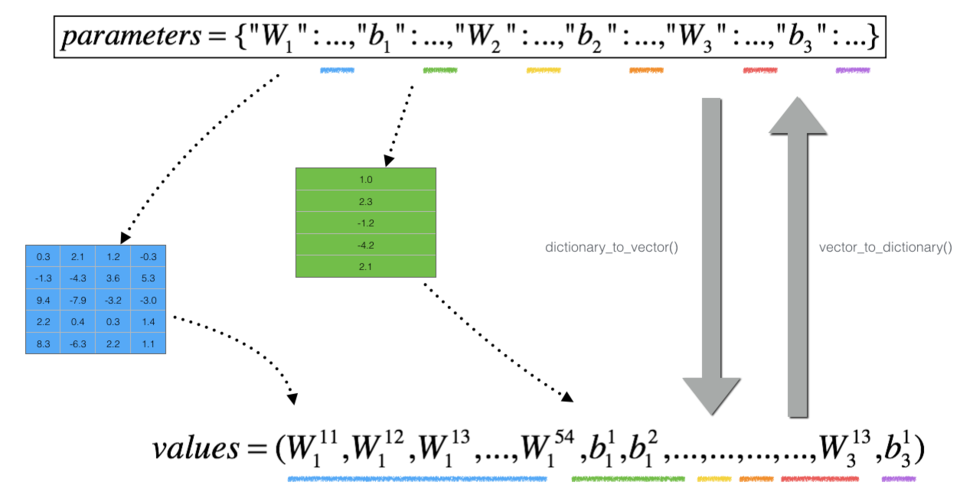
图2:dictionary_to_vector()和vector_to_dictionary()
你将在 gradient_check_n()中用到这些函数
我们还使用gradients_to_vector()将“gradients”字典转换为向量“grad”。
练习:实现gradient_check_n()。
说明:这是伪代码,可帮助你实现梯度检验。
For each i in num_parameters:
- 计算
J_plus [i]:- 将
设为
np.copy(parameters_values) - 将
设为
- 使用
forward_propagation_n(x, y, vector_to_dictionary())计算
- 将
- 计算
J_minus [i]:也是用 - 计算
因此,你将获得向量gradapprox,其中gradapprox[i]是相对于parameter_values[i]的梯度的近似值。现在,你可以将此gradapprox向量与反向传播中的梯度向量进行比较。就像一维情况(步骤1’,2’,3’)一样计算:
# GRADED FUNCTION: gradient_check_ndef gradient_check_n(parameters, gradients, X, Y, epsilon = 1e-7):# Set-up variablesparameters_values, _ = dictionary_to_vector(parameters)grad = gradients_to_vector(gradients)num_parameters = parameters_values.shape[0]J_plus = np.zeros((num_parameters, 1))J_minus = np.zeros((num_parameters, 1))gradapprox = np.zeros((num_parameters, 1))# Compute gradapproxfor i in range(num_parameters):# Compute J_plus[i]. Inputs: "parameters_values, epsilon". Output = "J_plus[i]".thetaplus = np.copy(parameters_values)thetaplus[i][0] = thetaplus[i][0] + epsilonJ_plus[i], _ = forward_propagation_n(X, Y, vector_to_dictionary(thetaplus))# Compute J_minus[i]. Inputs: "parameters_values, epsilon". Output = "J_minus[i]".thetaminus = np.copy(parameters_values)thetaminus[i][0] = thetaminus[i][0] - epsilonJ_minus[i], _ = forward_propagation_n(X, Y, vector_to_dictionary(thetaminus))# Compute gradapprox[i]gradapprox[i] = (J_plus[i] - J_minus[i]) / (2.* epsilon)# Compare gradapprox to backward propagation gradients by computing difference.numerator = np.linalg.norm(grad - gradapprox)denominator = np.linalg.norm(grad) + np.linalg.norm(gradapprox)difference = numerator / denominatorif difference > 1e-7:print ("\033[93m" + "There is a mistake in the backward propagation! difference = " + str(difference) + "\033[0m")else:print ("\033[92m" + "Your backward propagation works perfectly fine! difference = " + str(difference) + "\033[0m")return difference
X, Y, parameters = gradient_check_n_test_case()cost, cache = forward_propagation_n(X, Y, parameters)gradients = backward_propagation_n(X, Y, cache)difference = gradient_check_n(parameters, gradients, X, Y)
如果根据定义计算的梯度和反向传播计算的梯度差>1e-7,说明backward_propagation_n代码有错误!
注意
- 梯度检验很慢!用
%20-%20J(%5Ctheta%20-%20%5Cvarepsilon)%7D%7B2%20%5Cvarepsilon%7D#card=math&code=%5Cfrac%7B%5Cpartial%20J%7D%7B%5Cpartial%20%5Ctheta%7D%20%5Capprox%20%20%5Cfrac%7BJ%28%5Ctheta%20%2B%20%5Cvarepsilon%29%20-%20J%28%5Ctheta%20-%20%5Cvarepsilon%29%7D%7B2%20%5Cvarepsilon%7D&id=n2Rxg) 逼近梯度在计算上是很耗费资源的。因此,我们不会在训练期间的每次迭代中都进行梯度检验。只需检查几次梯度是否正确。
- 至少如我们介绍的那样,梯度检验不适用于dropout。通常,你将运行不带dropout的梯度检验算法以确保你的backprop是正确的,然后添加dropout。
4 总结
- 梯度检验可验证反向传播的梯度与梯度的数值近似值之间的接近度(使用正向传播进行计算)。
- 梯度检验很慢,因此我们不会在每次训练中都运行它。通常,你仅需确保其代码正确即可运行它,然后将其关闭并将backprop用于实际的学习过程。

若有收获,就点个赞吧
0 人点赞
