TensorFlow教程
在此笔记本中,你将学习在TensorFlow中执行以下操作:
- 初始化变量
- 创建自己的会话(session)
- 训练算法
- 实现神经网络
编程框架不仅可以缩短编码时间,而且有时还可以进行优化以加快代码速度。
1 探索Tensorflow库
首先,导入库:
import mathimport numpy as npimport h5pyimport matplotlib.pyplot as plt# import tensorflow as tfimport tensorflow.compat.v1 as tffrom tensorflow.python.framework import opsfrom tf_utils import load_dataset, random_mini_batches, convert_to_one_hot, predict%matplotlib inlinenp.random.seed(1)
现在,你已经导入了库,我们将引导你完成其不同的应用程序。你将从一个示例开始:计算一个训练数据的损失。
%20%3D%20(%5Chat%20y%5E%7B(i)%7D%20-%20y%5E%7B(i)%7D)%5E2%20%5Ctag%7B1%7D%0A#card=math&code=loss%20%3D%20%5Cmathcal%7BL%7D%28%5Chat%7By%7D%2C%20y%29%20%3D%20%28%5Chat%20y%5E%7B%28i%29%7D%20-%20y%5E%7B%28i%29%7D%29%5E2%20%5Ctag%7B1%7D%0A&id=iLwql)
tf.compat.v1.disable_eager_execution() # 此函数只能在创建任何图、运算或张量之前调用。它可以用于从TensorFlow 1.x到2.x的复杂迁移项目的程序开头。y_hat = tf.constant(36, name='y_hat') # Define y_hat constant. Set to 36.y = tf.constant(39, name='y') # Define y. Set to 39loss = tf.Variable((y - y_hat)**2, name='loss') # Create a variable for the lossinit = tf.global_variables_initializer() # When init is run later (session.run(init)),# the loss variable will be initialized and ready to be computedwith tf.Session() as session: # Create a session and print the outputsession.run(init) # Initializes the variablesprint(session.run(loss)) # Prints the loss
loss = 9
在TensorFlow中编写和运行程序包含以下步骤:
- 创建尚未执行的张量(变量)。
- 在这些张量之间编写操作。
- 初始化张量。
- 创建一个会话。
- 运行会话,这将运行你上面编写的操作。
因此,当我们为损失创建变量时,我们仅将损失定义为其他数量的函数,但没有验证其值。为了验证它,我们必须运行init = tf.global_variables_initializer()初始化损失变量,在最后一行中,我们终于能够验证loss的值并打印它。
现在让我们看一个简单的例子。运行下面的单元格:
a = tf.constant(2)b = tf.constant(10)c = tf.multiply(a,b)print(c) # Tensor("Mul:0", shape=(), dtype=int32)
看不到结果20!而是得到一个张量,是一个不具有shape属性且类型为“int32”的张量。你所做的所有操作都已放入“计算图”中,但你尚未运行此计算。为了实际将两个数字相乘,必须创建一个会话并运行它。
sess = tf.Session()print(sess.run(c)) #20
Great! 总而言之,记住要初始化变量,创建一个会话并在该会话中运行操作。
接下来,你还必须了解 placeholders(占位符)。占位符是一个对象,你只能稍后指定其值。
要为占位符指定值,你可以使用”feed dictionary”(feed_dict变量)传入值。在下面,我们为x创建了一个占位符,以允许我们稍后在运行会话时传递数字。
# Change the value of x in the feed_dictx = tf.placeholder(tf.int64, name = 'x')print(sess.run(2 * x, feed_dict = {x: 3})) # 6sess.close()
当你首次定义x时,不必为其指定值。占位符只是一个变量,你在运行会话时才将数据分配给该变量。也就是说你在运行会话时向这些占位符“提供数据”。
当你指定计算所需的操作时,你在告诉TensorFlow如何构造计算图。计算图可以具有一些占位符,你将在稍后指定它们的值。最后,在运行会话时,你要告诉TensorFlow执行计算图。
1.1 线性函数
让我们开始此编程练习,计算以下方程式:,其中
和
是随机矩阵,b是随机向量。
练习:计算 ,其中
和
是从随机正态分布中得到的,W的维度为(4,3),X的维度为(3,1),b的维度为(4,1)。例如,下面是定义维度为(3,1)的常量X的方法:
X = tf.constant(np.random.randn(3,1), name = "X")
你可能会发现以下函数很有用:
- tf.matmul(…, …)进行矩阵乘法
- tf.add(…, …)进行加法
- np.random.randn(…)随机初始化
# GRADED FUNCTION: linear_functiondef linear_function():"""Implements a linear function:Initializes W to be a random tensor of shape (4,3)Initializes X to be a random tensor of shape (3,1)Initializes b to be a random tensor of shape (4,1)Returns:result -- runs the session for Y = WX + b"""np.random.seed(1)### START CODE HERE ### (4 lines of code)X = tf.constant(np.random.randn(3, 1), name = "X")W = tf.constant(np.random.randn(4, 3), name = "W")b = tf.constant(np.random.randn(4, 1), name = "b")Y = tf.add(tf.matmul(W, X), b)### END CODE HERE #### Create the session using tf.Session() and run it with sess.run(...) on the variable you want to calculate### START CODE HERE ###sess = tf.Session()result = sess.run(Y)### END CODE HERE #### close the sessionsess.close()return result
print( "result = " + str(linear_function()))
预期输出:
result = [[-2.15657382]
[ 2.95891446]
[-1.08926781]
[-0.84538042]]
1.2 计算Sigmoid
Great!你刚刚实现了线性函数。Tensorflow提供了各种常用的神经网络函数,例如tf.sigmoid和tf.softmax。对于本练习,让我们计算输入的sigmoid函数值。
你将使用占位符变量x进行此练习。在运行会话时,应该使用feed字典传入输入z。在本练习中,你必须:
(i)创建一个占位符x;
(ii)使用tf.sigmoid定义计算Sigmoid所需的操作;
(iii)然后运行该会话
练习:实现下面的Sigmoid函数。你应该使用以下内容:
tf.placeholder(tf.float32, name = "...")tf.sigmoid(...)sess.run(..., feed_dict = {x: z})
注意,在tensorflow中创建和使用会话有两种典型的方法:
Method 1:
sess = tf.Session()# Run the variables initialization (if needed), run the operationsresult = sess.run(..., feed_dict = {...})sess.close() # Close the session
Method 2:
with tf.Session() as sess:# run the variables initialization (if needed), run the operationsresult = sess.run(..., feed_dict = {...})# This takes care of closing the session for you :)
# GRADED FUNCTION: sigmoiddef sigmoid(z):"""Computes the sigmoid of zArguments:z -- input value, scalar or vectorReturns:results -- the sigmoid of z"""### START CODE HERE ### ( approx. 4 lines of code)# Create a placeholder for x. Name it 'x'.x = tf.placeholder(tf.float32, name="x")# compute sigmoid(x)sigmoid = tf.sigmoid(x)# Create a session, and run it. Please use the method 2 explained above.# You should use a feed_dict to pass z's value to x.with tf.Session() as sess:result = sess.run(sigmoid, feed_dict={x:z})### END CODE HERE ###return result
print ("sigmoid(0) = " + str(sigmoid(0)))print ("sigmoid(12) = " + str(sigmoid(12)))
预期输出:
sigmoid(0) = 0.5
sigmoid(12) = 0.9999938
总而言之,你知道如何:
1.创建占位符
2.指定运算相对应的计算图
3.创建会话
4.如果需要指定占位符变量的值,使用feed字典运行会话。
1.3 计算损失
你还可以使用内置函数来计算神经网络的损失。因此,对于i=1…m,无需编写代码来将其作为%7D#card=math&code=a%5E%7B%5B2%5D%28i%29%7D&id=PJJ4E)和
%7D#card=math&code=y%5E%7B%28i%29%7D&id=CDGxs)的函数来计算:
%7D%20%5Clog%20a%5E%7B%20%5B2%5D%20(i)%7D%20%2B%20(1-y%5E%7B(i)%7D)%5Clog%20(1-a%5E%7B%20%5B2%5D%20(i)%7D%20)%5Clarge%20)%5Csmall%5Ctag%7B2%7D%20%0A#card=math&code=J%20%3D%20-%20%5Cfrac%7B1%7D%7Bm%7D%20%20%5Csum_%7Bi%20%3D%201%7D%5Em%20%20%5Clarge%20%28%20%5Csmall%20y%5E%7B%28i%29%7D%20%5Clog%20a%5E%7B%20%5B2%5D%20%28i%29%7D%20%2B%20%281-y%5E%7B%28i%29%7D%29%5Clog%20%281-a%5E%7B%20%5B2%5D%20%28i%29%7D%20%29%5Clarge%20%29%5Csmall%5Ctag%7B2%7D%20%0A&id=JdqH6)
你可以使用tensorflow的一行代码中做到这一点!
练习:实现交叉熵损失。你将使用的函数是:
tf.nn.sigmoid_cross_entropy_with_logits(logits = ..., labels = ...)
你的代码应输入z,计算出sigmoid(得到a),然后计算出交叉熵损失,所有这些操作都可以通过调用
tf.nn.sigmoid_cross_entropy_with_logits来完成:
%7D%20%5Clog%20%5Csigma(z%5E%7B%5B2%5D(i)%7D)%20%2B%20(1-y%5E%7B(i)%7D)%5Clog%20(1-%5Csigma(z%5E%7B%5B2%5D(i)%7D)%5Clarge%20)%5Csmall%5Ctag%7B2%7D%0A#card=math&code=-%5Cfrac%7B1%7D%7Bm%7D%20%20%5Csum_%7Bi%20%3D%201%7D%5Em%20%20%5Clarge%20%28%20%5Csmall%20y%5E%7B%28i%29%7D%20%5Clog%20%5Csigma%28z%5E%7B%5B2%5D%28i%29%7D%29%20%2B%20%281-y%5E%7B%28i%29%7D%29%5Clog%20%281-%5Csigma%28z%5E%7B%5B2%5D%28i%29%7D%29%5Clarge%20%29%5Csmall%5Ctag%7B2%7D%0A&id=aQUqc)
# GRADED FUNCTION: costdef cost(logits, labels):"""Computes the cost using the sigmoid cross entropyArguments:logits -- vector containing z, output of the last linear unit (before the final sigmoid activation)labels -- vector of labels y (1 or 0)Note: What we've been calling "z" and "y" in this class are respectively called "logits" and "labels"in the TensorFlow documentation. So logits will feed into z, and labels into y.Returns:cost -- runs the session of the cost (formula (2))"""# Create the placeholders for "logits" (z) and "labels" (y) (approx. 2 lines)z = tf.placeholder(tf.float32, name='z')y = tf.placeholder(tf.float32, name='y')# Use the loss function (approx. 1 line)loss = tf.nn.sigmoid_cross_entropy_with_logits(logits=z, labels=y)# Create a session (approx. 1 line). See method 1 above.sess = tf.Session()# Run the session (approx. 1 line).cost = sess.run(loss, feed_dict={z:logits, y:labels})# Close the session (approx. 1 line). See method 1 above.sess.close()### END CODE HERE ###return cost
logits = sigmoid(np.array([0.2,0.4,0.7,0.9]))cost = cost(logits, np.array([0,0,1,1]))print ("cost = " + str(cost))
预期输出 :
cost = [1.0053872 1.0366409 0.41385433 0.39956614]
1.4 使用独热(One Hot)编码
在深度学习中,很多时候你会得到一个y向量,其数字范围从0到C-1,其中C是类的数量。例如C是4,那么你可能具有以下y向量,你将需要按以下方式对其进行转换:
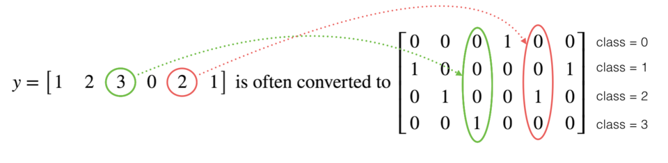
这称为独热编码,因为在转换后的表示形式中,每一列中的一个元素正好是“hot”(设为1)。要以numpy格式进行此转换,你可能需要编写几行代码。在tensorflow中,你可以只使用一行代码:
- tf.one_hot(labels, depth, axis)
练习:实现以下函数,以获取一个标签向量和类的总数,并返回一个独热编码。使用
tf.one_hot()来做到这一点。
# GRADED FUNCTION: one_hot_matrixdef one_hot_matrix(labels, C):"""Creates a matrix where the i-th row corresponds to the ith class number and the jth columncorresponds to the jth training example. So if example j had a label i. Then entry (i,j)will be 1.Arguments:labels -- vector containing the labelsC -- number of classes, the depth of the one hot dimensionReturns:one_hot -- one hot matrix"""### START CODE HERE #### Create a tf.constant equal to C (depth), name it 'C'. (approx. 1 line)C = tf.constant(C, name='C')# Use tf.one_hot, be careful with the axis (approx. 1 line)one_hot_matrix = tf.one_hot(labels, C, axis=0)# Create the session (approx. 1 line)sess = tf.Session()# Run the session (approx. 1 line)one_hot = sess.run(one_hot_matrix)# Close the session (approx. 1 line). See method 1 above.sess.close()### END CODE HERE ###return one_hot
labels = np.array([1,2,3,0,2,1])one_hot = one_hot_matrix(labels, C = 4)print (one_hot)
# 上面这个函数里面也是调用tf.one_hot,结果一样。写函数可能是为了让人熟悉tf的操作流程。one = tf.one_hot(labels,depth=4,axis=0)sess = tf.Session()ones = sess.run(one)sess.close()print(ones)
预期输出:
one_hot = [[0. 0. 0. 1. 0. 0.]
[1. 0. 0. 0. 0. 1.]
[0. 1. 0. 0. 1. 0.]
[0. 0. 1. 0. 0. 0.]]
1.5 使用0和1初始化
现在,你将学习如何初始化0和1的向量。 你将要调用的函数是tf.ones()。要使用零初始化,可以改用tf.zeros()。这些函数采用一个维度,并分别返回一个包含0和1的维度数组。
使用Tensorflow构建你的第一个神经网络
在这一部分作业中,你将使用tensorflow构建神经网络。请记住,实现tensorflow模型包含两个部分:
- 创建计算图
- 运行计算图
让我们深入研究你要解决的问题!
2.0 问题陈述:SIGNS 数据集
一个下午,我们决定和一些朋友一起用计算机来解密手语。我们花了几个小时在白墙前拍照,并提出了以下数据集。现在,你的工作就是构建一种算法,以帮助语音障碍者和不懂手语的人的交流。
- 训练集:1080张图片(64 x 64像素)的手势表示从0到5的数字(每个数字180张图片)。
- 测试集:120张图片(64 x 64像素)的手势表示从0到5的数字(每个数字20张图片)。
请注意,这是SIGNS数据集的子集。完整的数据集包含更多的手势。
这是每个数字的示例,以及如何解释标签的方式。这些是原始图片,然后我们将图像分辨率降低到64 x 64像素。
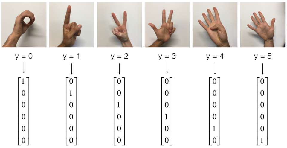
图 1:SIGNS数据集
运行以下代码以加载数据集。
# Loading the datasetX_train_orig, Y_train_orig, X_test_orig, Y_test_orig, classes = load_dataset()X_train_orig.shape, Y_train_orig.shape
((1080, 64, 64, 3), (1, 1080))
更改下面的索引并运行单元格以可视化数据集中的一些示例。
# Example of a pictureindex = 0plt.imshow(X_train_orig[index])print ("y = " + str(np.squeeze(Y_train_orig[:, index])))
y = 5

通常先将图像数据集展平,然后除以255以对其进行归一化。最重要的是将每个标签转换为一个独热向量,如图1所示。运行下面的单元格即可转化。
# Flatten the training and test imagesX_train_flatten = X_train_orig.reshape(X_train_orig.shape[0], -1).TX_test_flatten = X_test_orig.reshape(X_test_orig.shape[0], -1).T# Normalize image vectorsX_train = X_train_flatten/255.X_test = X_test_flatten/255.# Convert training and test labels to one hot matricesY_train = convert_to_one_hot(Y_train_orig, 6)Y_test = convert_to_one_hot(Y_test_orig, 6)print ("number of training examples = " + str(X_train.shape[1]))print ("number of test examples = " + str(X_test.shape[1]))print ("X_train shape: " + str(X_train.shape))print ("Y_train shape: " + str(Y_train.shape))print ("X_test shape: " + str(X_test.shape))print ("Y_test shape: " + str(Y_test.shape))
number of training examples = 1080number of test examples = 120X_train shape: (12288, 1080)Y_train shape: (6, 1080)X_test shape: (12288, 120)Y_test shape: (6, 120)
注意 12288 = ,每个图像均为正方形,64 x 64像素,其中3为RGB颜色。请确保理解这些数据的维度意义,然后再继续。
你的目标是建立一种能够高精度识别符号的算法。为此,你将构建一个tensorflow模型,该模型与你先前在numpy中为猫识别构建的tensorflow模型几乎相同(但现在使用softmax输出)。这是将numpy实现的模型与tensorflow进行比较的好机会。
模型为LINEAR-> RELU-> LINEAR-> RELU-> LINEAR-> SOFTMAX 。 SIGMOID输出层已转换为SOFTMAX。SOFTMAX层将SIGMOID应用到两个以上的类。
2.1 创建占位符
你的第一个任务是为X和X创建占位符,方便你以后在运行会话时传递训练数据。
练习:实现以下函数以在tensorflow中创建占位符。
# GRADED FUNCTION: create_placeholdersdef create_placeholders(n_x, n_y):"""Creates the placeholders for the tensorflow session.Arguments:n_x -- scalar, size of an image vector (num_px * num_px = 64 * 64 * 3 = 12288)n_y -- scalar, number of classes (from 0 to 5, so -> 6)Returns:X -- placeholder for the data input, of shape [n_x, None] and dtype "float"Y -- placeholder for the input labels, of shape [n_y, None] and dtype "float"Tips:- You will use None because it let's us be flexible on the number of examples you will for the placeholders.In fact, the number of examples during test/train is different."""### START CODE HERE ### (approx. 2 lines)X = tf.placeholder(tf.float32, shape=[n_x, None])Y = tf.placeholder(tf.float32, shape=[n_y, None])### END CODE HERE ###return X, Y
X, Y = create_placeholders(12288, 6)print ("X = " + str(X))print ("Y = " + str(Y))
X = Tensor("Placeholder:0", shape=(12288, None), dtype=float32)Y = Tensor("Placeholder_1:0", shape=(6, None), dtype=float32)
预期输出:
X = Tensor(“Placeholder:0”, shape=(12288, ?), dtype=float32)
Y = Tensor(“Placeholder_1:0”, shape=(6, ?), dtype=float32)
2.2 初始化参数
你的第二个任务是初始化tensorflow中的参数。
练习:实现以下函数以初始化tensorflow中的参数。使用权重的Xavier初始化和偏差的零初始化。维度如下,对于W1和b1,你可以使用:
W1 = tf.get_variable("W1", [25,12288], initializer = tf.contrib.layers.xavier_initializer(seed = 1))b1 = tf.get_variable("b1", [25,1], initializer = tf.zeros_initializer())
请使用seed = 1来确保你的结果与我们的结果相符。
注:the TF2 replacement for tf.contrib.layers.xavier_initializer() is tf.keras.initializers.glorot_normal(Xavier and Glorot are 2 names for the same initializer algorithm) documentation link.
# GRADED FUNCTION: initialize_parametersdef initialize_parameters():"""Initializes parameters to build a neural network with tensorflow. The shapes are:W1 : [25, 12288]b1 : [25, 1]W2 : [12, 25]b2 : [12, 1]W3 : [6, 12]b3 : [6, 1]Returns:parameters -- a dictionary of tensors containing W1, b1, W2, b2, W3, b3"""tf.set_random_seed(1) # so that your "random" numbers match ours### START CODE HERE ### (approx. 6 lines of code)W1 = tf.get_variable('W1', [25,12288], initializer=tf.keras.initializers.glorot_normal(seed = 1))b1 = tf.get_variable('b1', [25,1], initializer=tf.zeros_initializer())W2 = tf.get_variable('W2', [12,25], initializer=tf.keras.initializers.glorot_normal(seed = 1))b2 = tf.get_variable('b2', [12,1], initializer=tf.zeros_initializer())W3 = tf.get_variable('W3', [6,12], initializer=tf.keras.initializers.glorot_normal(seed = 1))b3 = tf.get_variable('b3', [6,1], initializer=tf.zeros_initializer())### END CODE HERE ###parameters = {"W1": W1,"b1": b1,"W2": W2,"b2": b2,"W3": W3,"b3": b3}return parameters
tf.reset_default_graph()with tf.Session() as sess:parameters = initialize_parameters()print("W1 = " + str(parameters["W1"]))print("b1 = " + str(parameters["b1"]))print("W2 = " + str(parameters["W2"]))print("b2 = " + str(parameters["b2"]))
W1 = <tf.Variable 'W1:0' shape=(25, 12288) dtype=float32>b1 = <tf.Variable 'b1:0' shape=(25, 1) dtype=float32>W2 = <tf.Variable 'W2:0' shape=(12, 25) dtype=float32>b2 = <tf.Variable 'b2:0' shape=(12, 1) dtype=float32>
预期输出:
W1 =
b1 =
W2 =
b2 =
如预期的那样,尚未对参数进行验证。
2.3 Tensorflow中的正向传播
你现在将在tensorflow中实现正向传播模块。该函数将接收参数字典,并将完成正向传递。你将使用的函数是:
tf.add(...,...)进行加法tf.matmul(...,...)进行矩阵乘法tf.nn.relu(...)以应用ReLU激活
问题:实现神经网络的正向传递。我们为你注释了numpy等式,以便你可以将tensorflow实现与numpy实现进行比较。重要的是要注意,前向传播在z3处停止。原因是在tensorflow中,最后的线性层输出作为计算损失函数的输入。因此,你不需要a3!
# GRADED FUNCTION: forward_propagationdef forward_propagation(X, parameters):"""Implements the forward propagation for the model: LINEAR -> RELU -> LINEAR -> RELU -> LINEAR -> SOFTMAXArguments:X -- input dataset placeholder, of shape (input size, number of examples)parameters -- python dictionary containing your parameters "W1", "b1", "W2", "b2", "W3", "b3"the shapes are given in initialize_parametersReturns:Z3 -- the output of the last LINEAR unit"""# Retrieve the parameters from the dictionary "parameters"W1 = parameters['W1']b1 = parameters['b1']W2 = parameters['W2']b2 = parameters['b2']W3 = parameters['W3']b3 = parameters['b3']### START CODE HERE ### (approx. 5 lines) # Numpy Equivalents:Z1 = tf.add(tf.matmul(W1,X),b1) # Z1 = np.dot(W1, X) + b1A1 = tf.nn.relu(Z1) # A1 = relu(Z1)Z2 = tf.add(tf.matmul(W2,A1),b2) # Z2 = np.dot(W2, A1) + b2A2 = tf.nn.relu(Z2) # A2 = relu(Z2)Z3 = tf.add(tf.matmul(W3,A2),b3) # Z3 = np.dot(W3,A2) + b3### END CODE HERE ###return Z3
tf.reset_default_graph()with tf.Session() as sess:X, Y = create_placeholders(12288, 6)parameters = initialize_parameters()Z3 = forward_propagation(X, parameters)print("Z3 = " + str(Z3))
Z3 = Tensor("Add_2:0", shape=(6, None), dtype=float32)
预期输出:
Z3 = Tensor(“Add_2:0”, shape=(6, ?), dtype=float32)
你可能已经注意到,正向传播不会输出任何缓存。当我们开始进行传播时,你将在下面理解为什么。
2.4 计算损失
如前所述,使用以下方法很容易计算损失:
tf.reduce_mean(tf.nn.softmax_cross_entropy_with_logits(logits = ..., labels = ...))
问题:实现以下损失函数。
- 重要的是要知道
tf.nn.softmax_cross_entropy_with_logits的”logits“和”labels“输入应具有一样的维度(数据数,类别数)。 因此,我们为你转换了Z3和Y。 - 此外,
tf.reduce_mean是对所以数据进行求和。
# GRADED FUNCTION: compute_costdef compute_cost(Z3, Y):"""Computes the costArguments:Z3 -- output of forward propagation (output of the last LINEAR unit), of shape (6, number of examples)Y -- "true" labels vector placeholder, same shape as Z3Returns:cost - Tensor of the cost function"""# to fit the tensorflow requirement for tf.nn.softmax_cross_entropy_with_logits(...,...)logits = tf.transpose(Z3)labels = tf.transpose(Y)### START CODE HERE ### (1 line of code)cost = tf.reduce_mean(tf.nn.softmax_cross_entropy_with_logits(logits=logits, labels=labels))### END CODE HERE ###return cost
tf.reset_default_graph()with tf.Session() as sess:X, Y = create_placeholders(12288, 6)parameters = initialize_parameters()Z3 = forward_propagation(X, parameters)cost = compute_cost(Z3, Y)print("cost = " + str(cost))
cost = Tensor("Mean:0", shape=(), dtype=float32)
预期输出:
cost = Tensor(“Mean:0”, shape=(), dtype=float32)
2.5 反向传播和参数更新
所有反向传播和参数更新均可使用1行代码完成,将这部分合并到模型中非常容易。
计算损失函数之后,你将创建一个”optimizer“对象。运行tf.session时,必须与损失一起调用此对象。调用时,它将使用所选方法和学习率对给定的损失执行优化。
例如,对于梯度下降,优化器将是:
optimizer = tf.train.GradientDescentOptimizer(learning_rate = learning_rate).minimize(cost)
要进行优化,你可以执行以下操作:
_ , c = sess.run([optimizer, cost], feed_dict={X: minibatch_X, Y: minibatch_Y})
通过相反顺序的tensorflow图来计算反向传播。从损失到输入。
注意编码时,我们经常使用_作为“throwaway”变量来存储以后不再需要使用的值。这里_代表了我们不需要的optimizer的评估值(而 c 代表了 cost变量的值)。
2.6 建立模型
现在,将它们组合在一起!
练习:调用之前实现的函数构建完整模型。
def model(X_train, Y_train, X_test, Y_test, learning_rate = 0.0001,num_epochs = 1500, minibatch_size = 32, print_cost = True):"""Implements a three-layer tensorflow neural network: LINEAR->RELU->LINEAR->RELU->LINEAR->SOFTMAX.Arguments:X_train -- training set, of shape (input size = 12288, number of training examples = 1080)Y_train -- test set, of shape (output size = 6, number of training examples = 1080)X_test -- training set, of shape (input size = 12288, number of training examples = 120)Y_test -- test set, of shape (output size = 6, number of test examples = 120)learning_rate -- learning rate of the optimizationnum_epochs -- number of epochs of the optimization loopminibatch_size -- size of a minibatchprint_cost -- True to print the cost every 100 epochsReturns:parameters -- parameters learnt by the model. They can then be used to predict."""ops.reset_default_graph() # to be able to rerun the model without overwriting tf variablestf.set_random_seed(1) # to keep consistent resultsseed = 3 # to keep consistent results(n_x, m) = X_train.shape # (n_x: input size, m : number of examples in the train set)n_y = Y_train.shape[0] # n_y : output sizecosts = [] # To keep track of the cost# Create Placeholders of shape (n_x, n_y)# X = tf.placeholder(tf.float32, shape=[n_x, None])# Y = tf.placeholder(tf.float32, shape=[n_y, None])X, Y = create_placeholders(n_x, n_y)# Initialize parametersparameters = initialize_parameters()# Forward propagation: Build the forward propagation in the tensorflow graphZ3 = forward_propagation(X, parameters)# Cost function: Add cost function to tensorflow graphcost = compute_cost(Z3, Y)# Backpropagation: Define the tensorflow optimizer. Use an AdamOptimizer.### START CODE HERE ### (1 line)optimizer = tf.train.AdamOptimizer(learning_rate = learning_rate).minimize(cost)### END CODE HERE #### Initialize all the variablesinit = tf.global_variables_initializer()# Start the session to compute the tensorflow graphwith tf.Session() as sess:# Run the initializationsess.run(init)# Do the training loopfor epoch in range(num_epochs):epoch_cost = 0. # Defines a cost related to an epochnum_minibatches = int(m / minibatch_size) # number of minibatches of size minibatch_size in the train setseed = seed + 1minibatches = random_mini_batches(X_train, Y_train, minibatch_size, seed)for minibatch in minibatches:# Select a minibatch(minibatch_X, minibatch_Y) = minibatch# IMPORTANT: The line that runs the graph on a minibatch.# Run the session to execute the "optimizer" and the "cost", the feedict should contain a minibatch for (X,Y).### START CODE HERE ### (1 line)_ , minibatch_cost = sess.run([optimizer, cost], feed_dict={X: minibatch_X, Y: minibatch_Y})### END CODE HERE ###epoch_cost += minibatch_cost / num_minibatches# Print the cost every epochif print_cost == True and epoch % 100 == 0:print ("Cost after epoch %i: %f" % (epoch, epoch_cost))if print_cost == True and epoch % 5 == 0:costs.append(epoch_cost)# plot the costplt.plot(np.squeeze(costs))plt.ylabel('cost')plt.xlabel('iterations (per tens)')plt.title("Learning rate =" + str(learning_rate))plt.show()# lets save the parameters in a variableparameters = sess.run(parameters)print ("Parameters have been trained!")# Calculate the correct predictionscorrect_prediction = tf.equal(tf.argmax(Z3), tf.argmax(Y))# Calculate accuracy on the test setaccuracy = tf.reduce_mean(tf.cast(correct_prediction, "float"))print ("Train Accuracy:", accuracy.eval({X: X_train, Y: Y_train}))print ("Test Accuracy:", accuracy.eval({X: X_test, Y: Y_test}))return parameters
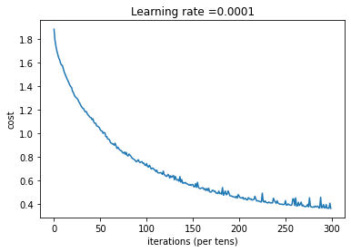
运行以下单元格来训练你的模型!在我们的机器上大约需要5分钟。 你的“100epoch后的损失”应为1.016458。如果不是,请不要浪费时间。单击笔记本电脑上方栏中的正方形(⬛),以中断训练,然后尝试更正你的代码。如果损失正确,请稍等片刻,然后在5分钟内回来!
parameters = model(X_train, Y_train, X_test, Y_test)
Cost after epoch 0: 1.882638Cost after epoch 100: 1.355498Cost after epoch 200: 1.132938Cost after epoch 300: 0.942660Cost after epoch 400: 0.807396Cost after epoch 500: 0.743592Cost after epoch 600: 0.643909Cost after epoch 700: 0.582018Cost after epoch 800: 0.536528Cost after epoch 900: 0.492420Cost after epoch 1000: 0.467958Cost after epoch 1100: 0.428083Cost after epoch 1200: 0.405582Cost after epoch 1300: 0.387620Cost after epoch 1400: 0.376748
预期输出:
Train Accuracy: 0.9990741
Test Accuracy: 0.725
Nice!你的算法可以识别出表示0到5之间数字的手势,准确度达到了71.7%。
评价:
- 你的模型足够强大,可以很好地拟合训练集。但是,鉴于训练和测试精度之间的差异,你可以尝试添加L2或dropout正则化以减少过拟合。
- 将会话视为训练模型的代码块。每次你在小批次上运行会话时,它都会训练参数。总的来说,你已经运行了该会话多次(1500个epoch),直到获得训练有素的参数为止。
2.7 使用自己的图像进行测试(可选练习)
祝贺你完成了此作业。现在,你可以拍张手的照片并查看模型的输出。要做到这一点:
1.单击此笔记本上部栏中的 “File” ,然后单击”Open”以在Coursera Hub上运行。
2.将图像添加到Jupyter Notebook的目录中,在 “images” 文件夹中
3.在以下代码中写下你的图片名称
4.运行代码,然后检查算法是否正确!
import scipyfrom PIL import Imagefrom scipy import ndimage## START CODE HERE ## (PUT YOUR IMAGE NAME)my_image = "thumbs_up.jpg"## END CODE HERE ### We preprocess your image to fit your algorithm.fname = my_imageimage = np.array(ndimage.imread(fname, flatten=False))my_image = scipy.misc.imresize(image, size=(64,64)).reshape((1, 64*64*3)).Tmy_image_prediction = predict(my_image, parameters)plt.imshow(image)print("Your algorithm predicts: y = " + str(np.squeeze(my_image_prediction)))
/opt/conda/lib/python3.6/site-packages/ipykernel_launcher.py:11: DeprecationWarning: `imread` is deprecated!`imread` is deprecated in SciPy 1.0.0.Use ``matplotlib.pyplot.imread`` instead.# This is added back by InteractiveShellApp.init_path()/opt/conda/lib/python3.6/site-packages/ipykernel_launcher.py:12: DeprecationWarning: `imresize` is deprecated!`imresize` is deprecated in SciPy 1.0.0, and will be removed in 1.3.0.Use Pillow instead: ``numpy.array(Image.fromarray(arr).resize())``.if sys.path[0] == '':Your algorithm predicts: y = 3
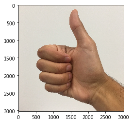
You indeed deserved a “thumbs-up” although as you can see the algorithm seems to classify it incorrectly. The reason is that the training set doesn’t contain any “thumbs-up”, so the model doesn’t know how to deal with it! We call that a “mismatched data distribution” and it is one of the various of the next course on “Structuring Machine Learning Projects”.
尽管你看到算法似乎对它进行了错误分类,但你确实值得“竖起大拇指”。原因是训练集不包含任何“竖起大拇指”,因此模型不知道如何处理! 我们称其为“数据不平衡”,它是下一章“构建机器学习项目”中的学习课程之一。
你应该记住:
- Tensorflow是深度学习中经常使用的编程框架
- Tensorflow中的两个主要对象类别是张量和运算符。
- 在Tensorflow中进行编码时,你必须执行以下步骤:
- 创建一个包含张量(变量,占位符…)和操作(tf.matmul,tf.add,…)的计算图
- 创建会话
- 初始化会话
- 运行会话以执行计算图 - 你可以像在model()中看到的那样多次执行计算图
- 在“优化器”对象上运行会话时,将自动完成反向传播和优化。

若有收获,就点个赞吧
0 人点赞
