关系拟合(回归)
建立数据集
import torchimport torch.nn.functional as F # 激活函数import matplotlib.pyplot as plt# torch.manual_seed(1) # reproduciblex = torch.unsqueeze(torch.linspace(-1, 1, 100), dim=1) # x data (tensor), shape=(100, 1)y = x.pow(2) + 0.2*torch.rand(x.size()) # noisy y data (tensor), shape=(100, 1# plt.scatter(x.data.numpy(), y.data.numpy())# plt.show()
建立神经网络
建立一个神经网络我们可以直接运用 torch 中的体系. 先定义所有的层属性(init()), 然后再一层层搭建(forward(x))层于层的关系链接.
class Net(torch.nn.Module): # 继承 torch 的 Moduledef __init__(self, n_feature, n_hidden, n_output):super(Net, self).__init__() # 继承 __init__ 功能# 定义每层用什么样的形式self.hidden = torch.nn.Linear(n_feature, n_hidden) # 隐藏层线性输出self.predict = torch.nn.Linear(n_hidden, n_output) # 输出层线性输出def forward(self, x): # 这同时也是 Module 中的 forward 功能# 正向传播输入值, 神经网络分析出输出值x = F.relu(self.hidden(x)) # 激励函数(隐藏层的线性值)x = self.predict(x) # 输出值return xnet = Net(n_feature=1, n_hidden=10, n_output=1)print(net) # net 的结构"""Net ((hidden): Linear (1 -> 10)(predict): Linear (10 -> 1))"""
训练网络
# optimizer 是训练的工具optimizer = torch.optim.SGD(net.parameters(), lr=0.01) # 传入 net 的所有参数, 学习率loss_func = torch.nn.MSELoss() # 预测值和真实值的误差计算公式 (均方差)for t in range(100):prediction = net(x) # 喂给 net 训练数据 x, 输出预测值loss = loss_func(prediction, y) # 计算两者的误差optimizer.zero_grad() # 清空上一步的残余更新参数值loss.backward() # 误差反向传播, 计算参数更新值optimizer.step() # 将参数更新值施加到 net 的 parameters 上
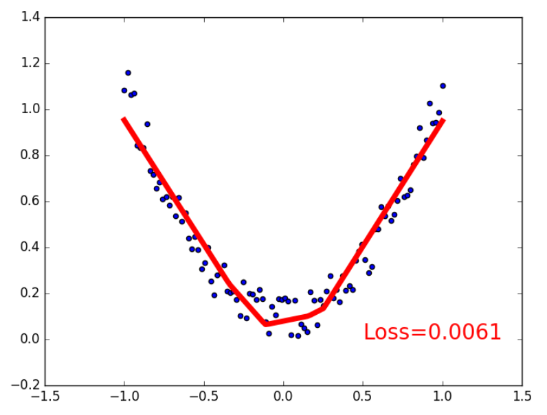
训练过程可视化
在for循环里添加画图功能。
plt.ion() # something about plottingfor t in range(200):prediction = net(x) # input x and predict based on xloss = loss_func(prediction, y) # must be (1. nn output, 2. target)optimizer.zero_grad() # clear gradients for next trainloss.backward() # backpropagation, compute gradientsoptimizer.step() # apply gradientsif t % 5 == 0:# plot and show learning processplt.cla()plt.scatter(x.data.numpy(), y.data.numpy())plt.plot(x.data.numpy(), prediction.data.numpy(), 'r-', lw=5)plt.text(0.5, 0, 'Loss=%.4f' % loss.data.numpy(), fontdict={'size': 20, 'color': 'red'})plt.pause(0.1)plt.ioff()plt.show()
分类
建立数据集
我们创建一些假数据来模拟真实的情况. 比如两个二次分布的数据, 不过他们的均值都不一样。
import torchimport matplotlib.pyplot as plt# 假数据n_data = torch.ones(100, 2) # 数据的基本形态x0 = torch.normal(2*n_data, 1) # 类型0 x data (tensor), shape=(100, 2)y0 = torch.zeros(100) # 类型0 y data (tensor), shape=(100, )x1 = torch.normal(-2*n_data, 1) # 类型1 x data (tensor), shape=(100, 1)y1 = torch.ones(100) # 类型1 y data (tensor), shape=(100, )# 注意 x, y 数据的数据形式是一定要像下面一样分为FloatTensor和LongTensor (torch.cat 是在合并数据),这是pytorch默认的形式x = torch.cat((x0, x1), 0).type(torch.FloatTensor) # FloatTensor = 32-bit floatingy = torch.cat((y0, y1), ).type(torch.LongTensor) # LongTensor = 64-bit integer# plt.scatter(x.data.numpy()[:, 0], x.data.numpy()[:, 1], c=y.data.numpy(), s=100, lw=0, cmap='RdYlGn')# plt.show()# 画图plt.scatter(x.data.numpy(), y.data.numpy())plt.show()
建立神经网络
这个和我们在前面 regression 的时候的神经网络基本没差,直接复制过来。
import torchimport torch.nn.functional as F # 激励函数都在这class Net(torch.nn.Module): # 继承 torch 的 Moduledef __init__(self, n_feature, n_hidden, n_output):super(Net, self).__init__() # 继承 __init__ 功能self.hidden = torch.nn.Linear(n_feature, n_hidden) # 隐藏层线性输出self.out = torch.nn.Linear(n_hidden, n_output) # 输出层线性输出def forward(self, x):# 正向传播输入值, 神经网络分析出输出值x = F.relu(self.hidden(x)) # 激励函数(隐藏层的线性值)x = self.out(x) # 输出值, 但是这个不是预测值, 预测值还需要再另外计算return xnet = Net(n_feature=2, n_hidden=10, n_output=2) # 几个类别就几个 outputprint(net) # net 的结构
训练网络
# optimizer 是训练的工具optimizer = torch.optim.SGD(net.parameters(), lr=0.02) # 传入 net 的所有参数, 学习率# 算误差的时候, 注意真实值!不是! one-hot 形式的, 而是1D Tensor, (batch,)# 但是预测值是2D tensor (batch, n_classes)loss_func = torch.nn.CrossEntropyLoss() # 分类问题常用的lossfor t in range(100):out = net(x) # 喂给 net 训练数据 x, 输出分析值loss = loss_func(out, y) # 计算两者的误差optimizer.zero_grad() # 清空上一步的残余更新参数值loss.backward() # 误差反向传播, 计算参数更新值optimizer.step() # 将参数更新值施加到 net 的 parameters 上
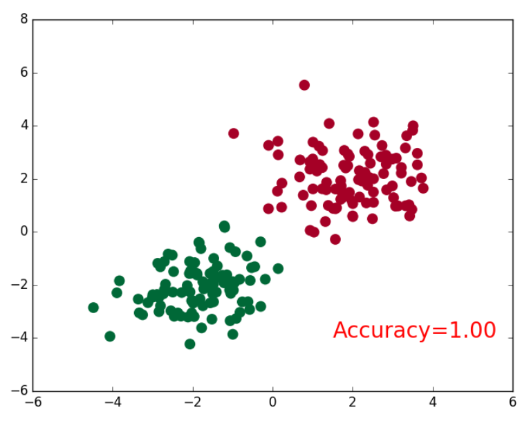
训练过程可视化
import matplotlib.pyplot as pltplt.ion()plt.show()for t in range(100):out = net(x) # 喂给 net 训练数据 x, 输出分析值loss = loss_func(out, y) # 计算两者的误差optimizer.zero_grad() # 清空上一步的残余更新参数值loss.backward()optimizer.step()# 画图if t % 2 == 0:plt.cla()# 过了一道 softmax 的激励函数后的最大概率才是预测值prediction = torch.max(F.softmax(out), 1)[1] # 索引0是最大值的值,索引1是它的位置pred_y = prediction.data.numpy().squeeze()target_y = y.data.numpy()plt.scatter(x.data.numpy()[:, 0], x.data.numpy()[:, 1], c=pred_y, s=100, lw=0, cmap='RdYlGn')accuracy = sum(pred_y == target_y)/200. # 预测中有多少和真实值一样plt.text(1.5, -4, 'Accuracy=%.2f' % accuracy, fontdict={'size': 20, 'color': 'red'})plt.pause(0.1)plt.ioff() # 停止画图plt.show()
快速搭建
不用像上面那样自己定义class Net(torch.nn.module),直接调用torch.nn.Sequential。效果是一样的。
net2 = torch.nn.Sequential(torch.nn.Linear(1, 10),torch.nn.ReLU(),torch.nn.Linear(10, 1))print(net2)"""Sequential ((0): Linear (1 -> 10)(1): ReLU ()(2): Linear (10 -> 1))"""
保存网络
torch.manual_seed(1) # reproducible# 假数据x = torch.unsqueeze(torch.linspace(-1, 1, 100), dim=1) # x data (tensor), shape=(100, 1)y = x.pow(2) + 0.2*torch.rand(x.size()) # noisy y data (tensor), shape=(100, 1)def save():# 建网络net1 = torch.nn.Sequential(torch.nn.Linear(1, 10),torch.nn.ReLU(),torch.nn.Linear(10, 1))optimizer = torch.optim.SGD(net1.parameters(), lr=0.5)loss_func = torch.nn.MSELoss()# 训练for t in range(100):prediction = net1(x)loss = loss_func(prediction, y)optimizer.zero_grad()loss.backward()optimizer.step()
可以保存这整个网络,也可以只保存网络中的参数。
torch.save(net1, 'net.pkl') # 保存整个网络torch.save(net1.state_dict(), 'net_params.pkl') # 只保存网络中的参数 (速度快, 占内存少)
提取网络
2种方式:
net2 = torch.load('net.pkl') # 提取整个网络到net2,包括结构和参数net3.load_state_dict(torch.load('net_params.pkl')) # 提取网络参数到net3
举例,1.提取整个网络:
def restore_net():# restore entire net1 to net2net2 = torch.load('net.pkl')prediction = net2(x)
2.只提取参数:
def restore_params():# 新建一个同样的网络结构 net3net3 = torch.nn.Sequential(torch.nn.Linear(1, 10),torch.nn.ReLU(),torch.nn.Linear(10, 1))# 将保存的参数复制到 net3net3.load_state_dict(torch.load('net_params.pkl'))prediction = net3(x)
DataLoader
Torch 中提供了一种帮你整理你的数据结构的好东西, 叫做 DataLoader, 我们能用它来包装自己的数据, 进行批训练. 所以你要将自己的 (numpy array 或其他) 数据形式装换成 Tensor, 然后再放进这个包装器中. 使用 DataLoader 有什么好处呢? 就是他们帮你有效地迭代数据, 举例:
import torchimport torch.utils.data as Datatorch.manual_seed(1) # reproducibleBATCH_SIZE = 5 # 批训练的数据个数x = torch.linspace(1, 10, 10) # x data (torch tensor)y = torch.linspace(10, 1, 10) # y data (torch tensor)# 先转换成 torch 能识别的 Datasettorch_dataset = Data.TensorDataset(data_tensor=x, target_tensor=y)# 把 dataset 放入 DataLoader,将数据分批loader = Data.DataLoader(dataset=torch_dataset, # torch TensorDataset formatbatch_size=BATCH_SIZE, # mini batch sizeshuffle=True, # 要不要打乱数据 (打乱比较好)num_workers=2, # 多线程来读数据)for epoch in range(3): # 训练所有数据 3 次for step, (batch_x, batch_y) in enumerate(loader): # 每一步 loader 释放一小批数据用来学习# 假设这里就是你训练的地方...# 打出来一些数据print('Epoch: ', epoch, '| Step: ', step, '| batch x: ',batch_x.numpy(), '| batch y: ', batch_y.numpy())"""Epoch: 0 | Step: 0 | batch x: [ 6. 7. 2. 3. 1.] | batch y: [ 5. 4. 9. 8. 10.]Epoch: 0 | Step: 1 | batch x: [ 9. 10. 4. 8. 5.] | batch y: [ 2. 1. 7. 3. 6.]Epoch: 1 | Step: 0 | batch x: [ 3. 4. 2. 9. 10.] | batch y: [ 8. 7. 9. 2. 1.]Epoch: 1 | Step: 1 | batch x: [ 1. 7. 8. 5. 6.] | batch y: [ 10. 4. 3. 6. 5.]Epoch: 2 | Step: 0 | batch x: [ 3. 9. 2. 6. 7.] | batch y: [ 8. 2. 9. 5. 4.]Epoch: 2 | Step: 1 | batch x: [ 10. 4. 8. 1. 5.] | batch y: [ 1. 7. 3. 10. 6.]"""
加速训练-优化器
主要包括以下几种模式:
- Stochastic Gradient Descent (SGD)
- Momentum
- AdaGrad
- RMSProp
- Adam
建立数据集
```python import torch import torch.utils.data as Data import torch.nn.functional as F import matplotlib.pyplot as plt
torch.manual_seed(1) # reproducible
LR = 0.01 BATCH_SIZE = 32 EPOCH = 12
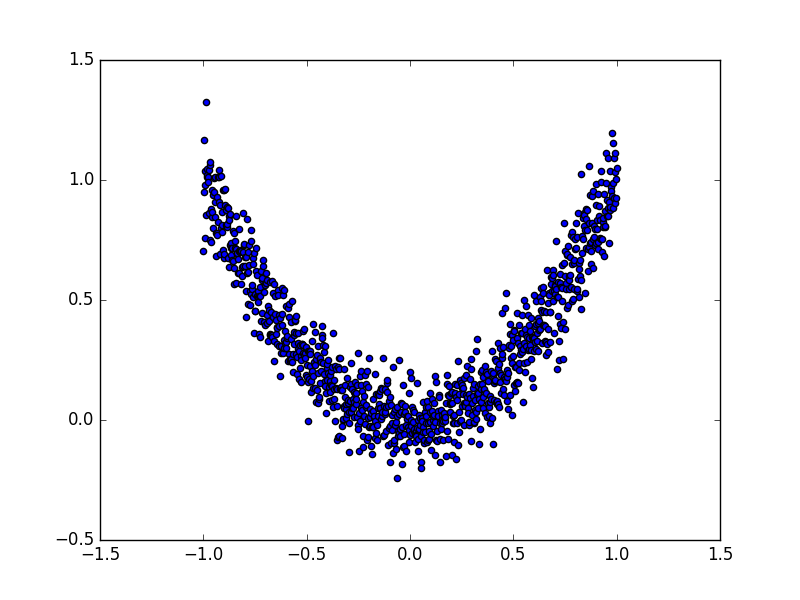
fake dataset
x = torch.unsqueeze(torch.linspace(-1, 1, 1000), dim=1) y = x.pow(2) + 0.1torch.normal(torch.zeros(x.size()))
plot dataset
plt.scatter(x.numpy(), y.numpy()) plt.show()
使用上节内容提到的 data loader
torch_dataset = Data.TensorDataset(x, y) loader = Data.DataLoader(dataset=torch_dataset, batch_size=BATCH_SIZE, shuffle=True, num_workers=2,)
<a name="iKImA"></a>## 建立神经网络```python# 默认的 network 形式class Net(torch.nn.Module):def __init__(self):super(Net, self).__init__()self.hidden = torch.nn.Linear(1, 20) # hidden layerself.predict = torch.nn.Linear(20, 1) # output layerdef forward(self, x):x = F.relu(self.hidden(x)) # activation function for hidden layerx = self.predict(x) # linear outputreturn x
优化器 Optimizer
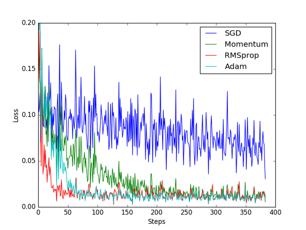
接下来在创建不同的优化器, 用来训练不同的网络. 并创建一个 loss_func 用来计算误差. 我们用几种常见的优化器, SGD, Momentum, RMSprop, Adam.
# 为每个优化器创建一个 netnet_SGD = Net()net_Momentum = Net()net_RMSprop = Net()net_Adam = Net()nets = [net_SGD, net_Momentum, net_RMSprop, net_Adam]# different optimizersopt_SGD = torch.optim.SGD(net_SGD.parameters(), lr=LR)opt_Momentum = torch.optim.SGD(net_Momentum.parameters(), lr=LR, momentum=0.8)opt_RMSprop = torch.optim.RMSprop(net_RMSprop.parameters(), lr=LR, alpha=0.9)opt_Adam = torch.optim.Adam(net_Adam.parameters(), lr=LR, betas=(0.9, 0.99))optimizers = [opt_SGD, opt_Momentum, opt_RMSprop, opt_Adam]loss_func = torch.nn.MSELoss()losses_his = [[], [], [], []] # 记录 training 时不同神经网络的 loss
训练 & 画图
for epoch in range(EPOCH):print('Epoch: ', epoch)for step, (b_x, b_y) in enumerate(loader):# 对每个优化器, 优化属于他的神经网络for net, opt, l_his in zip(nets, optimizers, losses_his):output = net(b_x) # get output for every netloss = loss_func(output, b_y) # compute loss for every netopt.zero_grad() # clear gradients for next trainloss.backward() # backpropagation, compute gradientsopt.step() # apply gradientsl_his.append(loss.data.numpy()) # loss recoderlabels = ['SGD', 'Momentum', 'RMSprop', 'Adam']for i, l_his in enumerate(losses_his):plt.plot(l_his,label=labels[i])plt.legend(loc='best')plt.xlabel('Steps')plt.ylabel('Loss')plt.ylim((0, 0.2))plt.show()
CNN-MNIST手写数据识别
下载MNIST数据
import torchimport torch.nn as nnimport torch.utils.data as Dataimport torchvision # 数据库模块import matplotlib.pyplot as plttorch.manual_seed(1) # reproducible# Hyper ParametersEPOCH = 1 # 训练整批数据多少次, 为了节约时间, 我们只训练一次BATCH_SIZE = 50LR = 0.001 # 学习率DOWNLOAD_MNIST = True # 如果你已经下载好了mnist数据就写上 False# Mnist 手写数字train_data = torchvision.datasets.MNIST(root='./mnist/', # 保存或者提取位置train=True, # this is training datatransform=torchvision.transforms.ToTensor(), # 把像素值从0~255压缩到 0~1download=DOWNLOAD_MNIST, # 下载数据, 已有的话不会再下)
torchvision.transforms.ToTensor() 转换 PIL.Image or numpy.ndarray 成torch.FloatTensor (C x H x W), 训练的时候 normalize 成 [0.0, 1.0] 区间.
同样, 我们除了训练数据, 还给一些测试数据, 测试看看它有没有训练好.
test_data = torchvision.datasets.MNIST(root='./mnist/', train=False)# 批训练 50samples, 1 channel, 28x28 (50, 1, 28, 28)train_loader = Data.DataLoader(dataset=train_data, batch_size=BATCH_SIZE, shuffle=True)# 为了节约时间, 我们测试时只测试前2000个test_x = torch.unsqueeze(test_data.test_data, dim=1).type(torch.FloatTensor)[:2000]/255. # shape from (2000, 28, 28) to (2000, 1, 28, 28), value in range(0,1)test_y = test_data.test_labels[:2000]
CNN模型
和以前一样, 我们用一个 class 来建立 CNN 模型. 这个 CNN 整体流程是 卷积(Conv2d) -> 激励函数(ReLU) -> 池化, 向下采样 (MaxPooling) -> 再来一遍 -> 展平多维的卷积成的特征图 -> 接入全连接层 (Linear) -> 输出
class CNN(nn.Module):def __init__(self):super(CNN, self).__init__()self.conv1 = nn.Sequential( # input shape (1, 28, 28)nn.Conv2d(in_channels=1, # input height, 输入通道数out_channels=16, # n_filters, 输出通道数(filter个数)kernel_size=5, # filter sizestride=1,padding=2,), # output shape (16, 28, 28)nn.ReLU(), # activationnn.MaxPool2d(kernel_size=2), # 在 2x2 空间里向下采样, output shape (16, 14, 14))self.conv2 = nn.Sequential( # input shape (16, 14, 14)nn.Conv2d(16, 32, 5, 1, 2), # output shape (32, 14, 14)nn.ReLU(), # activationnn.MaxPool2d(2), # output shape (32, 7, 7))self.out = nn.Linear(32 * 7 * 7, 10) # fully connected layer, output 10 classesdef forward(self, x):x = self.conv1(x)x = self.conv2(x)x = x.view(x.size(0), -1) # 展平多维的卷积图成 (batch_size, 32 * 7 * 7)output = self.out(x)return outputcnn = CNN()print(cnn) # net architecture"""CNN ((conv1): Sequential ((0): Conv2d(1, 16, kernel_size=(5, 5), stride=(1, 1), padding=(2, 2))(1): ReLU ()(2): MaxPool2d (size=(2, 2), stride=(2, 2), dilation=(1, 1)))(conv2): Sequential ((0): Conv2d(16, 32, kernel_size=(5, 5), stride=(1, 1), padding=(2, 2))(1): ReLU ()(2): MaxPool2d (size=(2, 2), stride=(2, 2), dilation=(1, 1)))(out): Linear (1568 -> 10))"""
训练
optimizer = torch.optim.Adam(cnn.parameters(), lr=LR) # optimize all cnn parametersloss_func = nn.CrossEntropyLoss() # the target label is not one-hotted# training and testingfor epoch in range(EPOCH):for step, (b_x, b_y) in enumerate(train_loader): # 分配 batch data, normalize x when iterate train_loaderoutput = cnn(b_x) # cnn outputloss = loss_func(output, b_y) # cross entropy lossoptimizer.zero_grad() # clear gradients for this training steploss.backward() # backpropagation, compute gradientsoptimizer.step() # apply gradients
最后我们再来取10个数据, 看看预测的值到底对不对:
test_output = cnn(test_x[:10])pred_y = torch.max(test_output, 1)[1].data.numpy().squeeze()print(pred_y, 'prediction number')print(test_y[:10].numpy(), 'real number')"""[7 2 1 0 4 1 4 9 5 9] prediction number[7 2 1 0 4 1 4 9 5 9] real number"""
RNN-MNIST(分类)
导入包和数据,设置超参数:
import torchfrom torch import nnimport torchvision.datasets as dsetsimport torchvision.transforms as transformsimport matplotlib.pyplot as plttorch.manual_seed(1) # reproducible# Hyper ParametersEPOCH = 1 # 训练整批数据多少次, 为了节约时间, 我们只训练一次BATCH_SIZE = 64TIME_STEP = 28 # rnn 时间步数 / 图片高度INPUT_SIZE = 28 # rnn 每步输入值 / 图片每行像素# 也就是每个时间步处理一行像素LR = 0.01 # learning rateDOWNLOAD_MNIST = True # 如果你已经下载好了mnist数据就写上 Fasle# Mnist 手写数字train_data = torchvision.datasets.MNIST(root='./mnist/', # 保存或者提取位置train=True, # this is training datatransform=torchvision.transforms.ToTensor(), # 转换 PIL.Image or numpy.ndarray 成# torch.FloatTensor (C x H x W), 训练的时候 normalize 成 [0.0, 1.0] 区间download=DOWNLOAD_MNIST,)test_data = torchvision.datasets.MNIST(root='./mnist/', train=False)# 批训练 50samples, 1 channel, 28x28 (50, 1, 28, 28)train_loader = Data.DataLoader(dataset=train_data, batch_size=BATCH_SIZE, shuffle=True)# 为了节约时间, 我们测试时只测试前2000个test_x = torch.unsqueeze(test_data.test_data, dim=1).type(torch.FloatTensor)[:2000]/255. # shape from (2000, 28, 28) to (2000, 1, 28, 28), value in range(0,1)test_y = test_data.test_labels[:2000]
LSTM模型
和以前一样, 我们用一个 class 来建立 RNN 模型. 这个 RNN 整体流程是
- (input0, state0) -> LSTM -> (output0, state1);
- (input1, state1) -> LSTM -> (output1, state2);
- …
- (inputN, stateN)-> LSTM -> (outputN, stateN+1);
outputN -> Linear -> prediction. 通过LSTM分析每一时刻的值, 并且将这一时刻和前面时刻的理解合并在一起, 生成当前时刻对前面数据的理解或记忆. 传递这种理解给下一时刻分析. ```python class RNN(nn.Module): def init(self):
super(RNN, self).__init__()self.rnn = nn.LSTM( # LSTM 效果要比 nn.RNN() 好多了input_size=28, # 图片每行的数据像素点hidden_size=64, # rnn hidden unitnum_layers=1, # 有几层 RNN layersbatch_first=True, # input & output 会是以 batch size 为第一维度的特征集 e.g. (batch, time_step, input_size))self.out = nn.Linear(64, 10) # 输出层
def forward(self, x):
# x shape (batch, time_step, input_size)# r_out shape (batch, time_step, output_size)# h_n shape (n_layers, batch, hidden_size) LSTM 有两个 hidden states, h_n 是分线, h_c 是主线# h_c shape (n_layers, batch, hidden_size)r_out, (h_n, h_c) = self.rnn(x, None) # None 表示 hidden state 会用全0的 state# 选取最后一个时间点的 r_out 输出# 这里 r_out[:, -1, :] 的值也是 h_n 的值out = self.out(r_out[:, -1, :])return out
rnn = RNN() print(rnn) “”” RNN ( (rnn): LSTM(28, 64, batch_first=True) (out): Linear (64 -> 10) ) “””
<a name="BjUmu"></a>## 训练我们将图片数据看成一个时间上的连续数据, 每一行的像素点都是这个时刻的输入, 读完整张图片就是从上而下的读完了每行的像素点. 然后我们就可以拿出 RNN 在最后一步的分析值判断图片是哪一类了.```pythonoptimizer = torch.optim.Adam(rnn.parameters(), lr=LR) # optimize all parametersloss_func = nn.CrossEntropyLoss() # the target label is not one-hotted# training and testingfor epoch in range(EPOCH):for step, (x, b_y) in enumerate(train_loader): # gives batch datab_x = x.view(-1, 28, 28) # reshape x to (batch, time_step, input_size)output = rnn(b_x) # rnn outputloss = loss_func(output, b_y) # cross entropy lossoptimizer.zero_grad() # clear gradients for this training steploss.backward() # backpropagation, compute gradientsoptimizer.step() # apply gradients
RNN 回归
RNN模型
class RNN(nn.Module):def __init__(self):super(RNN, self).__init__()self.rnn = nn.RNN( # 这回一个普通的 RNN 就能胜任input_size=1,hidden_size=32, # rnn hidden unitnum_layers=1, # 有几层 RNN layersbatch_first=True, # input & output 会是以 batch size 为第一维度的特征集 e.g. (batch, time_step, input_size))self.out = nn.Linear(32, 1)def forward(self, x, h_state): # 因为 hidden state 是连续的, 所以我们要一直传递这一个 state# x (batch, time_step, input_size)# h_state (n_layers, batch, hidden_size)# r_out (batch, time_step, output_size)r_out, h_state = self.rnn(x, h_state) # h_state 也要作为 RNN 的一个输入outs = [] # 保存所有时间点的预测值for time_step in range(r_out.size(1)): # 对每一个时间点计算 outputouts.append(self.out(r_out[:, time_step, :]))return torch.stack(outs, dim=1), h_staternn = RNN()print(rnn)"""RNN ((rnn): RNN(1, 32, batch_first=True)(out): Linear (32 -> 1))"""
其实熟悉 RNN 的朋友应该知道, forward 过程中的对每个时间点求输出还有一招使得计算量比较小的. 不过上面的内容主要是为了呈现 PyTorch 在动态构图上的优势, 所以我用了一个 for loop 来搭建那套输出系统. 下面介绍一个替换方式. 使用 reshape 的方式整批计算.
def forward(self, x, h_state):r_out, h_state = self.rnn(x, h_state)r_out = r_out.view(-1, 32)outs = self.out(r_out)return outs.view(-1, 32, TIME_STEP), h_state
训练
我们使用 x 作为输入的 sin 值, 然后 y 作为想要拟合的输出, cos 值. 因为他们两条曲线是存在某种关系的, 所以我们就能用 sin 来预测 cos. rnn 会理解他们的关系, 并用里面的参数分析出来这个时刻 sin 曲线上的点如何对应上 cos 曲线上的点.
optimizer = torch.optim.Adam(rnn.parameters(), lr=LR) # optimize all rnn parametersloss_func = nn.MSELoss()h_state = None # 要使用初始 hidden state, 可以设成 Nonefor step in range(100):start, end = step * np.pi, (step+1)*np.pi # time steps# sin 预测 cossteps = np.linspace(start, end, 10, dtype=np.float32)x_np = np.sin(steps) # float32 for converting torch FloatTensory_np = np.cos(steps)x = torch.from_numpy(x_np[np.newaxis, :, np.newaxis]) # shape (batch, time_step, input_size)y = torch.from_numpy(y_np[np.newaxis, :, np.newaxis])prediction, h_state = rnn(x, h_state) # rnn 对于每个 step 的 prediction, 还有最后一个 step 的 h_state# !! 下一步十分重要 !!h_state = h_state.data # 要把 h_state 重新包装一下才能放入下一个 iteration, 不然会报错loss = loss_func(prediction, y) # cross entropy lossoptimizer.zero_grad() # clear gradients for this training steploss.backward() # backpropagation, compute gradientsoptimizer.step() # apply gradients
AutoEncode
原来有时神经网络要接受大量的输入信息, 比如输入信息是高清图片时, 输入信息量可能达到上千万, 让神经网络直接从上千万个信息源中学习是一件很吃力的工作. 所以, 何不压缩一下, 提取出原图片中的最具代表性的信息, 缩减输入信息量, 再把缩减过后的信息放进神经网络学习. 这样学习起来就简单轻松了. 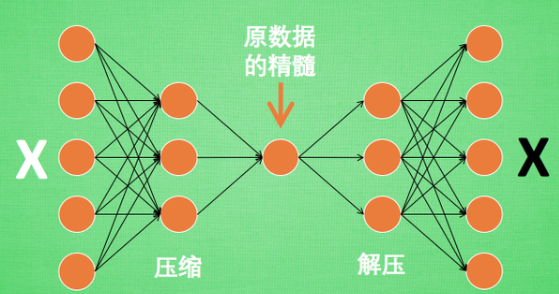
所以, 自编码就能在这时发挥作用. 通过将原数据白色的X 压缩, 解压 成黑色的X, 然后通过对比黑白 X ,求出预测误差, 进行反向传递, 逐步提升自编码的准确性. 训练好的自编码中间这一部分就是能总结原数据的精髓. 可以看出, 从头到尾, 我们只用到了输入数据 X, 并没有用到 X 对应的数据标签, 所以也可以说自编码是一种非监督学习. 到了真正使用自编码的时候. 通常只会用到自编码的压缩部分,也称为编码器。
如果你了解 PCA 主成分分析, 在提取主要特征时, 自编码和它一样,甚至超越了 PCA. 换句话说, 自编码 可以像 PCA 一样 给特征属性降维.
AutoEncoder 形式很简单, 分别是 encoder 和 decoder, 压缩和解压, 压缩后得到压缩的特征值, 再从压缩的特征值解压成原图片.
class AutoEncoder(nn.Module):def __init__(self):super(AutoEncoder, self).__init__()# 压缩self.encoder = nn.Sequential(nn.Linear(28*28, 128),nn.Tanh(),nn.Linear(128, 64),nn.Tanh(),nn.Linear(64, 12),nn.Tanh(),nn.Linear(12, 3), # 压缩成3个特征, 进行 3D 图像可视化)# 解压self.decoder = nn.Sequential(nn.Linear(3, 12),nn.Tanh(),nn.Linear(12, 64),nn.Tanh(),nn.Linear(64, 128),nn.Tanh(),nn.Linear(128, 28*28),nn.Sigmoid(), # 激励函数让输出值在 (0, 1))def forward(self, x):encoded = self.encoder(x)decoded = self.decoder(encoded)return encoded, decodedautoencoder = AutoEncoder()optimizer = torch.optim.Adam(autoencoder.parameters(), lr=LR)loss_func = nn.MSELoss()for epoch in range(EPOCH):for step, (x, b_label) in enumerate(train_loader):b_x = x.view(-1, 28*28) # batch x, shape (batch, 28*28)b_y = x.view(-1, 28*28) # batch y, shape (batch, 28*28)encoded, decoded = autoencoder(b_x)loss = loss_func(decoded, b_y) # mean square erroroptimizer.zero_grad() # clear gradients for this training steploss.backward() # backpropagation, compute gradientsoptimizer.step() # apply gradients

若有收获,就点个赞吧
0 人点赞
