优化算法

优化算法

到目前为止，你一直使用梯度下降来更新参数并使损失降至最低。在本笔记本中，你将学习更多高级的优化方法，以加快学习速度，甚至可以使你的损失函数的获得更低的最终值。一个好的优化算法可以使需要训练几天的网络，训练仅仅几个小时就能获得良好的结果。

在训练的每个步骤中，你都按照一定的方向更新参数，以尝试到达最低点。

符号：与往常一样， $【HW】L2W2-梯度下降的优化 - 图1$ da适用于任何变量a。

首先，请运行以下代码以导入所需的库。

import numpy as np
import matplotlib.pyplot as plt
import scipy.io
import math
import sklearn
import sklearn.datasets
from opt_utils import load_params_and_grads, initialize_parameters, forward_propagation, backward_propagation
from opt_utils import compute_cost, predict, predict_dec, plot_decision_boundary, load_dataset
from testCases import *
%matplotlib inline
plt.rcParams['figure.figsize'] = (7.0, 4.0) # set default size of plots
plt.rcParams['image.interpolation'] = 'nearest'
plt.rcParams['image.cmap'] = 'gray'

1 梯度下降

机器学习中一种简单的优化方法是梯度下降（gradient descent,GD）。当你对每个step中的所有 $【HW】L2W2-梯度下降的优化 - 图2$ 示例执行梯度计算步骤时，它也叫做“批量梯度下降”。

热身练习：实现梯度下降更新方法。对于 $【HW】L2W2-梯度下降的优化 - 图3$ ，梯度下降规则为：

$【HW】L2W2-梯度下降的优化 - 图4$

$【HW】L2W2-梯度下降的优化 - 图5$

其中L是层数， $【HW】L2W2-梯度下降的优化 - 图6$ 是学习率。所有参数都应存储在 parameters字典中。请注意，迭代器l在for 循环中从0开始，而第一个参数是 $【HW】L2W2-梯度下降的优化 - 图7$ 和 $【HW】L2W2-梯度下降的优化 - 图8$ 。编码时需要将l 转换为l+1。

# GRADED FUNCTION: update_parameters_with_gd
def update_parameters_with_gd(parameters, grads, learning_rate):
    L = len(parameters) // 2 # number of layers in the neural networks
    # Update rule for each parameter
    for l in range(L):
        parameters["W" + str(l+1)] = parameters["W" + str(l+1)] - learning_rate*grads["dW" + str(l+1)]
        parameters["b" + str(l+1)] = parameters["b" + str(l+1)] -learning_rate*grads["db" + str(l+1)]
    return parameters

它的一种变体是随机梯度下降（SGD），它相当于mini版的批次梯度下降，其中每个mini-batch只有一个数据示例。刚刚实现的更新规则不会更改。不同的是，SGD一次仅在一个训练数据上计算梯度，而不是在整个训练集合上计算梯度。下面的代码示例说明了随机梯度下降和（批量）梯度下降之间的区别。

(Batch) Gradient Descent:

X = data_input
Y = labels
parameters = initialize_parameters(layers_dims)
for i in range(0, num_iterations):
    # Forward propagation
    a, caches = forward_propagation(X, parameters)
    # Compute cost.
    cost = compute_cost(a, Y)
    # Backward propagation.
    grads = backward_propagation(a, caches, parameters)
    # Update parameters.
    parameters = update_parameters(parameters, grads)

Stochastic Gradient Descent:

X = data_input
Y = labels
parameters = initialize_parameters(layers_dims)
for i in range(0, num_iterations):
    for j in range(0, m):
        # Forward propagation
        a, caches = forward_propagation(X[:,j], parameters)
        # Compute cost
        cost = compute_cost(a, Y[:,j])
        # Backward propagation
        grads = backward_propagation(a, caches, parameters)
        # Update parameters.
        parameters = update_parameters(parameters, grads)

对于随机梯度下降，在更新梯度之前，只使用1个训练样例。当训练集大时，SGD可以更新的更快。但是这些参数会向最小值“摆动”而不是平稳地收敛。下图是一个演示例子：

【HW】L2W2-梯度下降的优化 - 图9

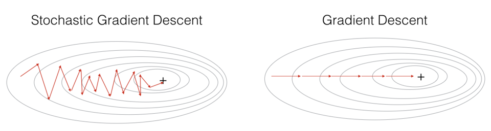
图 1: SGD vs GD
“+”表示损失的最小值。 SGD造成许多振荡以达到收敛。但是每个step中，计算SGD比使用GD更快，因为它仅使用一个训练示例（相对于GD的整个批次）。

实现SGD总共需要3个for循环：
1.迭代次数
2. $【HW】L2W2-梯度下降的优化 - 图10$ 个训练数据
3.各层上（要更新所有参数，从 $【HW】L2W2-梯度下降的优化 - 图11$ #card=math&code=%28W%5E%7B%5B1%5D%7D%2Cb%5E%7B%5B1%5D%7D%29&id=tF6bV)到 $【HW】L2W2-梯度下降的优化 - 图12$ #card=math&code=%28W%5E%7B%5BL%5D%7D%2Cb%5E%7B%5BL%5D%7D%29&id=EBVks))

小批量梯度下降法通常会得到更快的结果。通过小批量梯度下降，你可以遍历小批量，而不是遍历各个训练示例。

【HW】L2W2-梯度下降的优化 - 图13

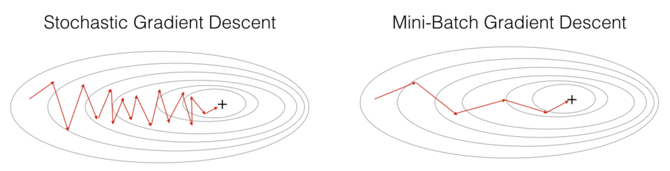
图 2：SGD vs Mini-Batch GD
“+”表示损失的最小值。在优化算法中使用mini-batch批处理通常可以加快优化速度。

你应该记住：

梯度下降，小批量梯度下降和随机梯度下降之间的差异是用于执行一个更新步骤的数据数量。
必须调整超参数学习率 $【HW】L2W2-梯度下降的优化 - 图14$ 。
在小批量的情况下，通常它会胜过梯度下降或随机梯度下降（尤其是训练集较大时）。

2 Mini-Batch 梯度下降

让我们学习如何从训练集（X，Y）中构建小批次数据。

分两个步骤：

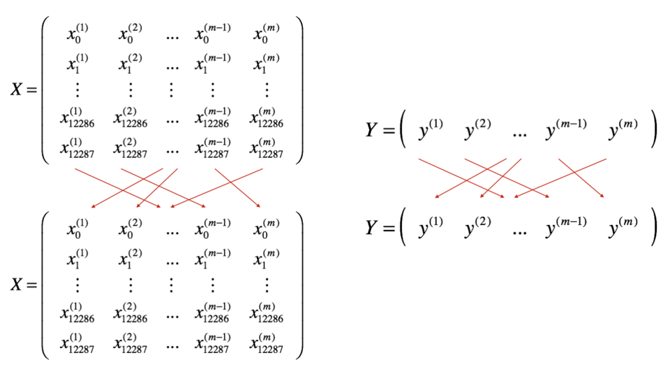
Shuffle：如下所示，创建训练集（X，Y）的随机打乱版本。X和Y中的每一列代表一个训练示例。注意，随机打乱是在X和Y之间同步完成的。这样，在随机打乱之后，X的 $【HW】L2W2-梯度下降的优化 - 图15$ 列就是对应于Y中 $【HW】L2W2-梯度下降的优化 - 图16$ 标签的示例。打乱步骤可确保该示例将随机分为不同小批。

【HW】L2W2-梯度下降的优化 - 图17

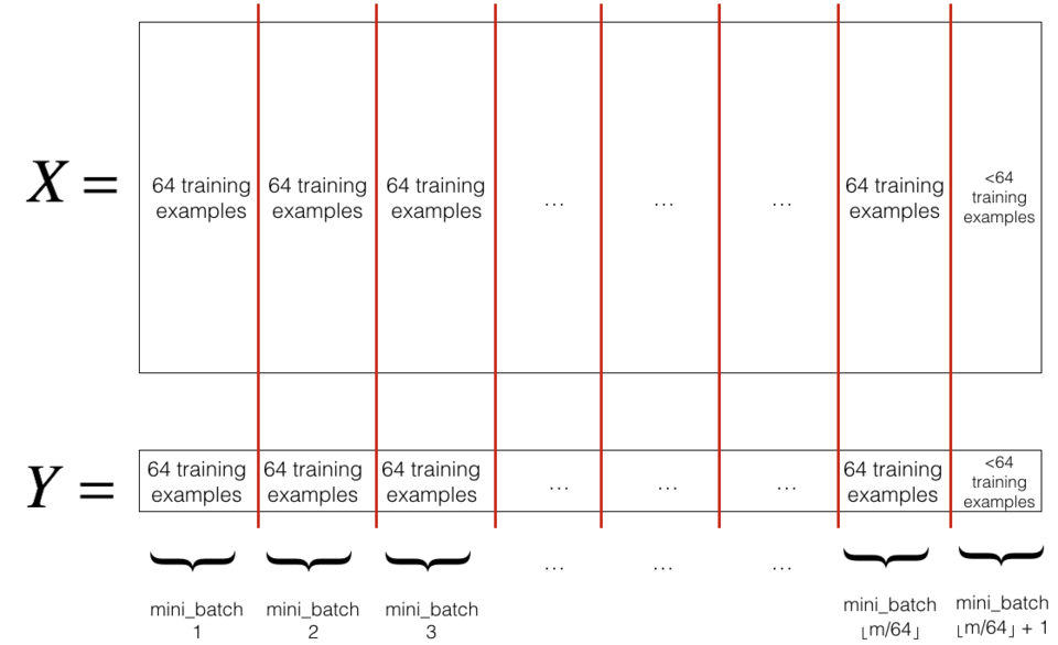
Partition：将打乱后的（X，Y）划分为大小为mini_batch_size（此处为64）的小批处理。请注意，训练示例的数量并不总是可以被mini_batch_size整除。最后的小批量可能较小，但是你不必担心，当最终的迷你批处理小于完整的mini_batch_size时，它将如下图所示：

【HW】L2W2-梯度下降的优化 - 图18

练习：实现random_mini_batches。我们为你编码好了shuffling部分。为了帮助你实现partitioning部分，我们为你提供了以下代码，用于选择 $【HW】L2W2-梯度下降的优化 - 图19$ 和 $【HW】L2W2-梯度下降的优化 - 图20$ 小批次的索引：

first_mini_batch_X = shuffled_X[:, 0 : mini_batch_size]
second_mini_batch_X = shuffled_X[:, mini_batch_size : 2 * mini_batch_size]
...

请注意，最后一个小批次的结果可能小于mini_batch_size=64。令 $【HW】L2W2-梯度下降的优化 - 图21$ 代表 $【HW】L2W2-梯度下降的优化 - 图22$ 向下舍入到最接近的整数（在Python中为math.floor（s））。如果示例总数不是mini_batch_size = 64的倍数，则将有 $【HW】L2W2-梯度下降的优化 - 图23$ 个带有完整示例的小批次，数量为64最终的一批次中的示例将是( $【HW】L2W2-梯度下降的优化 - 图24$ )。

# GRADED FUNCTION: random_mini_batches
def random_mini_batches(X, Y, mini_batch_size = 64, seed = 0):
    """
    Creates a list of random minibatches from (X, Y)
    Arguments:
    X -- input data, of shape (input size, number of examples)
    Y -- true "label" vector (1 for blue dot / 0 for red dot), of shape (1, number of examples)
    mini_batch_size -- size of the mini-batches, integer
    Returns:
    mini_batches -- list of synchronous (mini_batch_X, mini_batch_Y)
    """
    np.random.seed(seed)            # To make your "random" minibatches the same as ours
    m = X.shape[1]                  # number of training examples
    mini_batches = []
    # Step 1: Shuffle (X, Y)
    permutation = list(np.random.permutation(m))
    shuffled_X = X[:, permutation]
    shuffled_Y = Y[:, permutation].reshape((1,m))
    # Step 2: Partition (shuffled_X, shuffled_Y). Minus the end case.
    num_complete_minibatches = math.floor(m/mini_batch_size) # number of mini batches of size mini_batch_size in your partitionning
    for k in range(0, num_complete_minibatches):
        ### START CODE HERE ### (approx. 2 lines)
        mini_batch_X = shuffled_X[:, k * mini_batch_size : (k+1) * mini_batch_size]
        mini_batch_Y = shuffled_Y[:, k * mini_batch_size : (k+1) * mini_batch_size]
        ### END CODE HERE ###
        mini_batch = (mini_batch_X, mini_batch_Y)
        mini_batches.append(mini_batch)
    # Handling the end case (last mini-batch < mini_batch_size)
    if m % mini_batch_size != 0:
        ### START CODE HERE ### (approx. 2 lines)
        mini_batch_X = shuffled_X[:, num_complete_minibatches * mini_batch_size : m]
        mini_batch_Y = shuffled_Y[:, num_complete_minibatches * mini_batch_size : m]
        ### END CODE HERE ###
        mini_batch = (mini_batch_X, mini_batch_Y)
        mini_batches.append(mini_batch)
    return mini_batches

你应该记住：

Shuffling和Partitioning是构建小批次数据所需的两个步骤
通常选择2的幂作为最小批量大小，例如16、32、64、128。

3 Momentum

因为小批量梯度下降仅在看到示例的子集后才进行参数更新，所以更新的方向具有一定的差异，因此小批量梯度下降所采取的路径将“朝着收敛”振荡。利用冲量则可以减少这些振荡。

冲量考虑了过去的梯度以平滑更新。我们将先前梯度的“方向”存储在变量 $【HW】L2W2-梯度下降的优化 - 图25$ 中。这将是先前步骤中梯度的指数加权平均值，你也可以将 $【HW】L2W2-梯度下降的优化 - 图26$ 看作是下坡滚动的球的“速度”，根据山坡的坡度/坡度的方向来提高速度（和冲量）。

【HW】L2W2-梯度下降的优化 - 图27

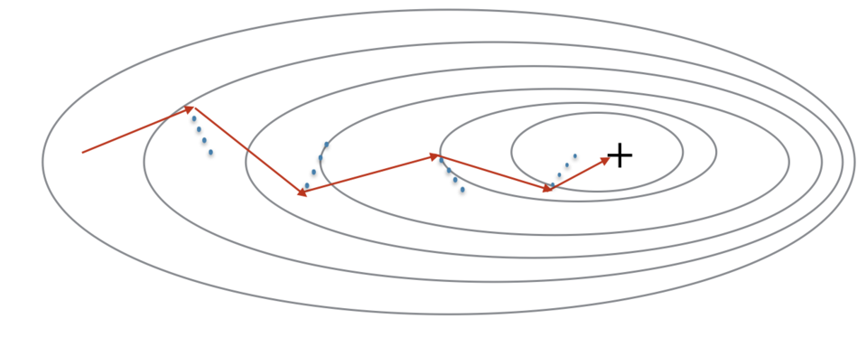
图 3：红色箭头显示了带冲量的小批次梯度下降步骤所采取的方向。蓝点表示每一步的梯度方向（相对于当前的小批量）。让梯度影响 $【HW】L2W2-梯度下降的优化 - 图28$ 而不是仅遵循梯度，然后朝 $【HW】L2W2-梯度下降的优化 - 图29$ 的方向迈出一步。

练习：初始化速度。速度 $【HW】L2W2-梯度下降的优化 - 图30$ 是一个Python字典，需要使用零数组进行初始化。它的键与grads词典中的键相同，即：
为 $【HW】L2W2-梯度下降的优化 - 图31$ ：

v["dW" + str(l+1)] = ... #(numpy array of zeros with the same shape as parameters["W" + str(l+1)])
v["db" + str(l+1)] = ... #(numpy array of zeros with the same shape as parameters["b" + str(l+1)])

注意：迭代器l在for循环中从0开始，而第一个参数是v[“dW1”]和v[“db1”]（在上标中为“1”）。这就是为什么我们在“for”循环中将l转换为l+1的原因。

# GRADED FUNCTION: initialize_velocity
def initialize_velocity(parameters):
    """
    Initializes the velocity as a python dictionary with:
                - keys: "dW1", "db1", ..., "dWL", "dbL" 
                - values: numpy arrays of zeros of the same shape as the corresponding gradients/parameters.
    Arguments:
    parameters -- python dictionary containing your parameters.
                    parameters['W' + str(l)] = Wl
                    parameters['b' + str(l)] = bl
    Returns:
    v -- python dictionary containing the current velocity.
                    v['dW' + str(l)] = velocity of dWl
                    v['db' + str(l)] = velocity of dbl
    """
    L = len(parameters) // 2 # number of layers in the neural networks
    v = {}
    # Initialize velocity
    for l in range(L):
        ### START CODE HERE ### (approx. 2 lines)
        v["dW" + str(l+1)] = np.zeros(parameters['W' + str(l+1)].shape)
        v["db" + str(l+1)] = np.zeros(parameters['b' + str(l+1)].shape)
        ### END CODE HERE ###
    return v

练习：实现带冲量的参数更新。冲量更新规则是，对于 $【HW】L2W2-梯度下降的优化 - 图32$ :

$【HW】L2W2-梯度下降的优化 - 图33$ %20dW%5E%7B%5Bl%5D%7D%20%5C%5C%0AW%5E%7B%5Bl%5D%7D%20%3D%20W%5E%7B%5Bl%5D%7D%20-%20%5Calpha%20v%7BdW%5E%7B%5Bl%5D%7D%7D%0A%5Cend%7Bcases%7D%5Ctag%7B3%7D%0A#card=math&code=%5Cbegin%7Bcases%7D%0Av%7BdW%5E%7B%5Bl%5D%7D%7D%20%3D%20%5Cbeta%20v%7BdW%5E%7B%5Bl%5D%7D%7D%20%2B%20%281%20-%20%5Cbeta%29%20dW%5E%7B%5Bl%5D%7D%20%5C%5C%0AW%5E%7B%5Bl%5D%7D%20%3D%20W%5E%7B%5Bl%5D%7D%20-%20%5Calpha%20v%7BdW%5E%7B%5Bl%5D%7D%7D%0A%5Cend%7Bcases%7D%5Ctag%7B3%7D%0A&id=qpI4c)

$【HW】L2W2-梯度下降的优化 - 图34$ %20db%5E%7B%5Bl%5D%7D%20%5C%5C%0Ab%5E%7B%5Bl%5D%7D%20%3D%20b%5E%7B%5Bl%5D%7D%20-%20%5Calpha%20v%7Bdb%5E%7B%5Bl%5D%7D%7D%20%0A%5Cend%7Bcases%7D%5Ctag%7B4%7D%0A#card=math&code=%5Cbegin%7Bcases%7D%0Av%7Bdb%5E%7B%5Bl%5D%7D%7D%20%3D%20%5Cbeta%20v%7Bdb%5E%7B%5Bl%5D%7D%7D%20%2B%20%281%20-%20%5Cbeta%29%20db%5E%7B%5Bl%5D%7D%20%5C%5C%0Ab%5E%7B%5Bl%5D%7D%20%3D%20b%5E%7B%5Bl%5D%7D%20-%20%5Calpha%20v%7Bdb%5E%7B%5Bl%5D%7D%7D%20%0A%5Cend%7Bcases%7D%5Ctag%7B4%7D%0A&id=nCO7B)

其中L是层数， $【HW】L2W2-梯度下降的优化 - 图35$ 是动量， $【HW】L2W2-梯度下降的优化 - 图36$ 是学习率。所有参数都应存储在parameters字典中。请注意，迭代器l在for循环中从0开始，而第一个参数是 $【HW】L2W2-梯度下降的优化 - 图37$ 和 $【HW】L2W2-梯度下降的优化 - 图38$ （在上标中为“1”）。因此，编码时需要将l转化至l+1。

# GRADED FUNCTION: update_parameters_with_momentum
def update_parameters_with_momentum(parameters, grads, v, beta, learning_rate):
    """
    Update parameters using Momentum
    Arguments:
    parameters -- python dictionary containing your parameters:
                    parameters['W' + str(l)] = Wl
                    parameters['b' + str(l)] = bl
    grads -- python dictionary containing your gradients for each parameters:
                    grads['dW' + str(l)] = dWl
                    grads['db' + str(l)] = dbl
    v -- python dictionary containing the current velocity:
                    v['dW' + str(l)] = ...
                    v['db' + str(l)] = ...
    beta -- the momentum hyperparameter, scalar
    learning_rate -- the learning rate, scalar
    Returns:
    parameters -- python dictionary containing your updated parameters 
    v -- python dictionary containing your updated velocities
    """
    L = len(parameters) // 2 # number of layers in the neural networks
    # Momentum update for each parameter
    for l in range(L):
        ### START CODE HERE ### (approx. 4 lines)
        # compute velocities
        v["dW" + str(l + 1)] = beta*v["dW" + str(l + 1)]+(1-beta)*grads['dW' + str(l+1)]
        v["db" + str(l + 1)] = beta*v["db" + str(l + 1)]+(1-beta)*grads['db' + str(l+1)]
        # update parameters
        parameters["W" + str(l + 1)] = parameters['W' + str(l+1)] - learning_rate*v["dW" + str(l + 1)] 
        parameters["b" + str(l + 1)] = parameters['b' + str(l+1)] - learning_rate*v["db" + str(l + 1)] 
        ### END CODE HERE ###
    return parameters, v

parameters, v = update_parameters_with_momentum(parameters, grads, v, beta = 0.9, learning_rate = 0.01)

W1 = [[ 1.62544598 -0.61290114 -0.52907334]
 [-1.07347112  0.86450677 -2.30085497]]
b1 = [[ 1.74493465]
 [-0.76027113]]
W2 = [[ 0.31930698 -0.24990073  1.4627996 ]
 [-2.05974396 -0.32173003 -0.38320915]
 [ 1.13444069 -1.0998786  -0.1713109 ]]
b2 = [[-0.87809283]
 [ 0.04055394]
 [ 0.58207317]]
v["dW1"] = [[-0.11006192  0.11447237  0.09015907]
 [ 0.05024943  0.09008559 -0.06837279]]
v["db1"] = [[-0.01228902]
 [-0.09357694]]
v["dW2"] = [[-0.02678881  0.05303555 -0.06916608]
 [-0.03967535 -0.06871727 -0.08452056]
 [-0.06712461 -0.00126646 -0.11173103]]
v["db2"] = [[0.02344157]
 [0.16598022]
 [0.07420442]]

注意：

速度用零初始化。因此，该算法将花费一些迭代来“提高”速度并开始采取更大的步骤。
如果 $【HW】L2W2-梯度下降的优化 - 图39$ ，则它变为没有冲量的标准梯度下降。

怎样选择 $【HW】L2W2-梯度下降的优化 - 图40$ ?

冲量 $【HW】L2W2-梯度下降的优化 - 图41$ 越大，更新越平滑，因为我们对过去的梯度的考虑也更多。但是，如果 $【HW】L2W2-梯度下降的优化 - 图42$ 太大，也可能使更新变得过于平滑。
$【HW】L2W2-梯度下降的优化 - 图43$ 的常用值范围是0.8到0.999。如果你不想调整它，则 $【HW】L2W2-梯度下降的优化 - 图44$ 通常是一个合理的默认值。
调整模型的最佳 $【HW】L2W2-梯度下降的优化 - 图45$ 可能需要尝试几个值，以了解在降低损失函数 $【HW】L2W2-梯度下降的优化 - 图46$ 的值方面最有效的方法。

你应该记住：

冲量将过去的梯度考虑在内，以平滑梯度下降的步骤。它可以应用于批量梯度下降，小批次梯度下降或随机梯度下降。
必须调整冲量超参数 $【HW】L2W2-梯度下降的优化 - 图47$ 和学习率 $【HW】L2W2-梯度下降的优化 - 图48$ 。

4 Adam

Adam是训练神经网络最有效的优化算法之一。它结合了RMSProp和Momentum的优点。

Adam原理
1.计算过去梯度的指数加权平均值，并将其存储在变量 $【HW】L2W2-梯度下降的优化 - 图49$ （使用偏差校正之前）和 $【HW】L2W2-梯度下降的优化 - 图50$ （使用偏差校正）中。
2.计算过去梯度的平方的指数加权平均值，并将其存储在变量 $【HW】L2W2-梯度下降的优化 - 图51$ （偏差校正之前）和 $【HW】L2W2-梯度下降的优化 - 图52$ （偏差校正中）中。
3.组合“1”和“2”的信息，在一个方向上更新参数。

对于 $【HW】L2W2-梯度下降的优化 - 图53$ ，更新规则为：

$【HW】L2W2-梯度下降的优化 - 图54$ %20%5Cfrac%7B%5Cpartial%20%5Cmathcal%7BJ%7D%20%7D%7B%20%5Cpartial%20W%5E%7B%5Bl%5D%7D%20%7D%20%5C%5C%0Av%5E%7Bcorrected%7D%7BdW%5E%7B%5Bl%5D%7D%7D%20%3D%20%5Cfrac%7Bv%7BdW%5E%7B%5Bl%5D%7D%7D%7D%7B1%20-%20(%5Cbeta1)%5Et%7D%20%5C%5C%0As%7BdW%5E%7B%5Bl%5D%7D%7D%20%3D%20%5Cbeta2%20s%7BdW%5E%7B%5Bl%5D%7D%7D%20%2B%20(1%20-%20%5Cbeta2)%20(%5Cfrac%7B%5Cpartial%20%5Cmathcal%7BJ%7D%20%7D%7B%5Cpartial%20W%5E%7B%5Bl%5D%7D%20%7D)%5E2%20%5C%5C%0As%5E%7Bcorrected%7D%7BdW%5E%7B%5Bl%5D%7D%7D%20%3D%20%5Cfrac%7Bs%7BdW%5E%7B%5Bl%5D%7D%7D%7D%7B1%20-%20(%5Cbeta_1)%5Et%7D%20%5C%5C%0AW%5E%7B%5Bl%5D%7D%20%3D%20W%5E%7B%5Bl%5D%7D%20-%20%5Calpha%20%5Cfrac%7Bv%5E%7Bcorrected%7D%7BdW%5E%7B%5Bl%5D%7D%7D%7D%7B%5Csqrt%7Bs%5E%7Bcorrected%7D%7BdW%5E%7B%5Bl%5D%7D%7D%7D%20%2B%20%5Cvarepsilon%7D%0A%5Cend%7Bcases%7D%0A#card=math&code=%5Cbegin%7Bcases%7D%0Av%7BdW%5E%7B%5Bl%5D%7D%7D%20%3D%20%5Cbeta1%20v%7BdW%5E%7B%5Bl%5D%7D%7D%20%2B%20%281%20-%20%5Cbeta1%29%20%5Cfrac%7B%5Cpartial%20%5Cmathcal%7BJ%7D%20%7D%7B%20%5Cpartial%20W%5E%7B%5Bl%5D%7D%20%7D%20%5C%5C%0Av%5E%7Bcorrected%7D%7BdW%5E%7B%5Bl%5D%7D%7D%20%3D%20%5Cfrac%7Bv%7BdW%5E%7B%5Bl%5D%7D%7D%7D%7B1%20-%20%28%5Cbeta_1%29%5Et%7D%20%5C%5C%0As%7BdW%5E%7B%5Bl%5D%7D%7D%20%3D%20%5Cbeta2%20s%7BdW%5E%7B%5Bl%5D%7D%7D%20%2B%20%281%20-%20%5Cbeta2%29%20%28%5Cfrac%7B%5Cpartial%20%5Cmathcal%7BJ%7D%20%7D%7B%5Cpartial%20W%5E%7B%5Bl%5D%7D%20%7D%29%5E2%20%5C%5C%0As%5E%7Bcorrected%7D%7BdW%5E%7B%5Bl%5D%7D%7D%20%3D%20%5Cfrac%7Bs%7BdW%5E%7B%5Bl%5D%7D%7D%7D%7B1%20-%20%28%5Cbeta_1%29%5Et%7D%20%5C%5C%0AW%5E%7B%5Bl%5D%7D%20%3D%20W%5E%7B%5Bl%5D%7D%20-%20%5Calpha%20%5Cfrac%7Bv%5E%7Bcorrected%7D%7BdW%5E%7B%5Bl%5D%7D%7D%7D%7B%5Csqrt%7Bs%5E%7Bcorrected%7D_%7BdW%5E%7B%5Bl%5D%7D%7D%7D%20%2B%20%5Cvarepsilon%7D%0A%5Cend%7Bcases%7D%0A&id=YkrPI)

其中：

t计算出Adam采取的步骤数
L是层数
$【HW】L2W2-梯度下降的优化 - 图55$ 和 $【HW】L2W2-梯度下降的优化 - 图56$ 是控制两个指数加权平均值的超参数。
$【HW】L2W2-梯度下降的优化 - 图57$ 是学习率
$【HW】L2W2-梯度下降的优化 - 图58$ 是一个很小的数字，以避免被零除

和之前一样，我们将所有参数存储在parameters字典中

练习：初始化跟踪过去信息的Adam变量 $【HW】L2W2-梯度下降的优化 - 图59$

说明：变量 $【HW】L2W2-梯度下降的优化 - 图60$ 是需要用零数组初始化的python字典。它们的key与grads的key相同。

# GRADED FUNCTION: initialize_adam
def initialize_adam(parameters) :
    """
    Initializes v and s as two python dictionaries with:
                - keys: "dW1", "db1", ..., "dWL", "dbL" 
                - values: numpy arrays of zeros of the same shape as the corresponding gradients/parameters.
    Arguments:
    parameters -- python dictionary containing your parameters.
                    parameters["W" + str(l)] = Wl
                    parameters["b" + str(l)] = bl
    Returns: 
    v -- python dictionary that will contain the exponentially weighted average of the gradient.
                    v["dW" + str(l)] = ...
                    v["db" + str(l)] = ...
    s -- python dictionary that will contain the exponentially weighted average of the squared gradient.
                    s["dW" + str(l)] = ...
                    s["db" + str(l)] = ...
    """
    L = len(parameters) // 2 # number of layers in the neural networks
    v = {}
    s = {}
    # Initialize v, s. Input: "parameters". Outputs: "v, s".
    for l in range(L):
    ### START CODE HERE ### (approx. 4 lines)
        v["dW" + str(l + 1)] = np.zeros(parameters["W" + str(l+1)].shape)
        v["db" + str(l + 1)] = np.zeros(parameters["b" + str(l+1)].shape)
        s["dW" + str(l + 1)] = np.zeros(parameters["W" + str(l+1)].shape)
        s["db" + str(l + 1)] = np.zeros(parameters["b" + str(l+1)].shape)
        ### END CODE HERE ###
    return v, s

练习：用Adam实现参数更新。回想一下一般的更新规则是，对于 $【HW】L2W2-梯度下降的优化 - 图61$ :

$【HW】L2W2-梯度下降的优化 - 图62$ %20%5Cfrac%7B%5Cpartial%20J%20%7D%7B%20%5Cpartial%20W%5E%7B%5Bl%5D%7D%20%7D%20%5C%5C%0Av%5E%7Bcorrected%7D%7BW%5E%7B%5Bl%5D%7D%7D%20%3D%20%5Cfrac%7Bv%7BW%5E%7B%5Bl%5D%7D%7D%7D%7B1%20-%20(%5Cbeta1)%5Et%7D%20%5C%5C%0As%7BW%5E%7B%5Bl%5D%7D%7D%20%3D%20%5Cbeta2%20s%7BW%5E%7B%5Bl%5D%7D%7D%20%2B%20(1%20-%20%5Cbeta2)%20(%5Cfrac%7B%5Cpartial%20J%20%7D%7B%5Cpartial%20W%5E%7B%5Bl%5D%7D%20%7D)%5E2%20%5C%5C%0As%5E%7Bcorrected%7D%7BW%5E%7B%5Bl%5D%7D%7D%20%3D%20%5Cfrac%7Bs%7BW%5E%7B%5Bl%5D%7D%7D%7D%7B1%20-%20(%5Cbeta_2)%5Et%7D%20%5C%5C%0AW%5E%7B%5Bl%5D%7D%20%3D%20W%5E%7B%5Bl%5D%7D%20-%20%5Calpha%20%5Cfrac%7Bv%5E%7Bcorrected%7D%7BW%5E%7B%5Bl%5D%7D%7D%7D%7B%5Csqrt%7Bs%5E%7Bcorrected%7D%7BW%5E%7B%5Bl%5D%7D%7D%7D%2B%5Cvarepsilon%7D%0A%5Cend%7Bcases%7D#card=math&code=%5Cbegin%7Bcases%7D%0Av%7BW%5E%7B%5Bl%5D%7D%7D%20%3D%20%5Cbeta1%20v%7BW%5E%7B%5Bl%5D%7D%7D%20%2B%20%281%20-%20%5Cbeta1%29%20%5Cfrac%7B%5Cpartial%20J%20%7D%7B%20%5Cpartial%20W%5E%7B%5Bl%5D%7D%20%7D%20%5C%5C%0Av%5E%7Bcorrected%7D%7BW%5E%7B%5Bl%5D%7D%7D%20%3D%20%5Cfrac%7Bv%7BW%5E%7B%5Bl%5D%7D%7D%7D%7B1%20-%20%28%5Cbeta_1%29%5Et%7D%20%5C%5C%0As%7BW%5E%7B%5Bl%5D%7D%7D%20%3D%20%5Cbeta2%20s%7BW%5E%7B%5Bl%5D%7D%7D%20%2B%20%281%20-%20%5Cbeta2%29%20%28%5Cfrac%7B%5Cpartial%20J%20%7D%7B%5Cpartial%20W%5E%7B%5Bl%5D%7D%20%7D%29%5E2%20%5C%5C%0As%5E%7Bcorrected%7D%7BW%5E%7B%5Bl%5D%7D%7D%20%3D%20%5Cfrac%7Bs%7BW%5E%7B%5Bl%5D%7D%7D%7D%7B1%20-%20%28%5Cbeta_2%29%5Et%7D%20%5C%5C%0AW%5E%7B%5Bl%5D%7D%20%3D%20W%5E%7B%5Bl%5D%7D%20-%20%5Calpha%20%5Cfrac%7Bv%5E%7Bcorrected%7D%7BW%5E%7B%5Bl%5D%7D%7D%7D%7B%5Csqrt%7Bs%5E%7Bcorrected%7D_%7BW%5E%7B%5Bl%5D%7D%7D%7D%2B%5Cvarepsilon%7D%0A%5Cend%7Bcases%7D&id=cYCaI)

注意:迭代器 l 在 for 循环中从0开始，而第一个参数是 $【HW】L2W2-梯度下降的优化 - 图63$ 和 $【HW】L2W2-梯度下降的优化 - 图64$ 。编码时需要将l转换为 l+1 。

# GRADED FUNCTION: update_parameters_with_adam
def update_parameters_with_adam(parameters, grads, v, s, t, learning_rate = 0.01,
                                beta1 = 0.9, beta2 = 0.999,  epsilon = 1e-8):
    """
    Update parameters using Adam
    Arguments:
    parameters -- python dictionary containing your parameters:
                    parameters['W' + str(l)] = Wl
                    parameters['b' + str(l)] = bl
    grads -- python dictionary containing your gradients for each parameters:
                    grads['dW' + str(l)] = dWl
                    grads['db' + str(l)] = dbl
    v -- Adam variable, moving average of the first gradient, python dictionary
    s -- Adam variable, moving average of the squared gradient, python dictionary
    learning_rate -- the learning rate, scalar.
    beta1 -- Exponential decay hyperparameter for the first moment estimates 
    beta2 -- Exponential decay hyperparameter for the second moment estimates 
    epsilon -- hyperparameter preventing division by zero in Adam updates
    Returns:
    parameters -- python dictionary containing your updated parameters 
    v -- Adam variable, moving average of the first gradient, python dictionary
    s -- Adam variable, moving average of the squared gradient, python dictionary
    """
    L = len(parameters) // 2                 # number of layers in the neural networks
    v_corrected = {}                         # Initializing first moment estimate, python dictionary
    s_corrected = {}                         # Initializing second moment estimate, python dictionary
    # Perform Adam update on all parameters
    for l in range(L):
        # Moving average of the gradients. Inputs: "v, grads, beta1". Output: "v".
        ### START CODE HERE ### (approx. 2 lines)
        v["dW" + str(l + 1)] = beta1*v["dW" + str(l + 1)] +(1-beta1)*grads['dW' + str(l+1)]
        v["db" + str(l + 1)] = beta1*v["db" + str(l + 1)] +(1-beta1)*grads['db' + str(l+1)]
        ### END CODE HERE ###
        # Compute bias-corrected first moment estimate. Inputs: "v, beta1, t". Output: "v_corrected".
        ### START CODE HERE ### (approx. 2 lines)
        v_corrected["dW" + str(l + 1)] = v["dW" + str(l + 1)]/(1-(beta1)**t)
        v_corrected["db" + str(l + 1)] = v["db" + str(l + 1)]/(1-(beta1)**t)
        ### END CODE HERE ###
        # Moving average of the squared gradients. Inputs: "s, grads, beta2". Output: "s".
        ### START CODE HERE ### (approx. 2 lines)
        s["dW" + str(l + 1)] =beta2*s["dW" + str(l + 1)] + (1-beta2)*(grads['dW' + str(l+1)]**2)
        s["db" + str(l + 1)] = beta2*s["db" + str(l + 1)] + (1-beta2)*(grads['db' + str(l+1)]**2)
        ### END CODE HERE ###
        # Compute bias-corrected second raw moment estimate. Inputs: "s, beta2, t". Output: "s_corrected".
        ### START CODE HERE ### (approx. 2 lines)
        s_corrected["dW" + str(l + 1)] =s["dW" + str(l + 1)]/(1-(beta2)**t)
        s_corrected["db" + str(l + 1)] = s["db" + str(l + 1)]/(1-(beta2)**t)
        ### END CODE HERE ###
        # Update parameters. Inputs: "parameters, learning_rate, v_corrected, s_corrected, epsilon". Output: "parameters".
        ### START CODE HERE ### (approx. 2 lines)
        parameters["W" + str(l + 1)] = parameters["W" + str(l + 1)]-learning_rate*(v_corrected["dW" + str(l + 1)]/np.sqrt( s_corrected["dW" + str(l + 1)]+epsilon))
        parameters["b" + str(l + 1)] = parameters["b" + str(l + 1)]-learning_rate*(v_corrected["db" + str(l + 1)]/np.sqrt( s_corrected["db" + str(l + 1)]+epsilon))
        ### END CODE HERE ###
    return parameters, v, s

现在，你学习了三种有效的优化算法（小批次梯度下降，冲量，Adam）。让我们使用每个优化器来实现一个模型，并观察其中的差异。

5 不同优化算法的模型对比

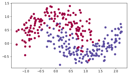
我们使用“moons”数据集来测试不同的优化方法。（该数据集被命名为“月亮”，因为两个类别的数据看起来有点像月牙。）

train_X, train_Y = load_dataset()

【HW】L2W2-梯度下降的优化 - 图65

我们已经实现了一个三层的神经网络。你将使用以下方法进行训练：

小批次 Gradient Descent:它将调用你的函数：
- update_parameters_with_gd（）
小批次冲量：它将调用你的函数：
- initialize_velocity（）和update_parameters_with_momentum（）
小批次 Adam：它将调用你的函数：
- initialize_adam（）和update_parameters_with_adam（）

def model(X, Y, layers_dims, optimizer, learning_rate = 0.0007, mini_batch_size = 64, beta = 0.9,
          beta1 = 0.9, beta2 = 0.999,  epsilon = 1e-8, num_epochs = 10000, print_cost = True):
    """
    3-layer neural network model which can be run in different optimizer modes.
    Arguments:
    X -- input data, of shape (2, number of examples)
    Y -- true "label" vector (1 for blue dot / 0 for red dot), of shape (1, number of examples)
    layers_dims -- python list, containing the size of each layer
    learning_rate -- the learning rate, scalar.
    mini_batch_size -- the size of a mini batch
    beta -- Momentum hyperparameter
    beta1 -- Exponential decay hyperparameter for the past gradients estimates 
    beta2 -- Exponential decay hyperparameter for the past squared gradients estimates 
    epsilon -- hyperparameter preventing division by zero in Adam updates
    num_epochs -- number of epochs
    print_cost -- True to print the cost every 1000 epochs
    Returns:
    parameters -- python dictionary containing your updated parameters 
    """
    L = len(layers_dims)             # number of layers in the neural networks
    costs = []                       # to keep track of the cost
    t = 0                            # initializing the counter required for Adam update
    seed = 10                        # For grading purposes, so that your "random" minibatches are the same as ours
    # Initialize parameters
    parameters = initialize_parameters(layers_dims)
    # Initialize the optimizer
    if optimizer == "gd":
        pass # no initialization required for gradient descent
    elif optimizer == "momentum":
        v = initialize_velocity(parameters)
    elif optimizer == "adam":
        v, s = initialize_adam(parameters)
    # Optimization loop
    for i in range(num_epochs):
        # Define the random minibatches. We increment the seed to reshuffle differently the dataset after each epoch
        seed = seed + 1
        minibatches = random_mini_batches(X, Y, mini_batch_size, seed)
        for minibatch in minibatches:
            # Select a minibatch
            (minibatch_X, minibatch_Y) = minibatch
            # Forward propagation
            a3, caches = forward_propagation(minibatch_X, parameters)
            # Compute cost
            cost = compute_cost(a3, minibatch_Y)
            # Backward propagation
            grads = backward_propagation(minibatch_X, minibatch_Y, caches)
            # Update parameters
            if optimizer == "gd":
                parameters = update_parameters_with_gd(parameters, grads, learning_rate)
            elif optimizer == "momentum":
                parameters, v = update_parameters_with_momentum(parameters, grads, v, beta, learning_rate)
            elif optimizer == "adam":
                t = t + 1 # Adam counter
                parameters, v, s = update_parameters_with_adam(parameters, grads, v, s,
                                                               t, learning_rate, beta1, beta2,  epsilon)
        # Print the cost every 1000 epoch
        if print_cost and i % 1000 == 0:
            print ("Cost after epoch %i: %f" %(i, cost))
        if print_cost and i % 100 == 0:
            costs.append(cost)
    # plot the cost
    plt.plot(costs)
    plt.ylabel('cost')
    plt.xlabel('epochs (per 100)')
    plt.title("Learning rate = " + str(learning_rate))
    plt.show()
    return parameters

现在，你将依次使用3种优化方法来运行此神经网络。

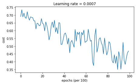
5.1 小批量梯度下降

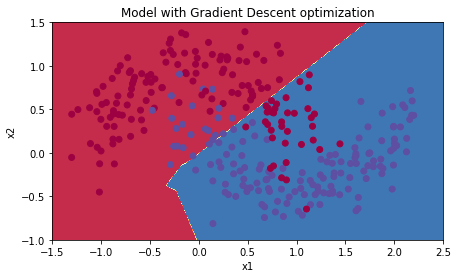
运行以下代码以查看模型如何进行小批量梯度下降。

# train 3-layer model
layers_dims = [train_X.shape[0], 5, 2, 1]
parameters = model(train_X, train_Y, layers_dims, optimizer = "gd")
# Predict
predictions = predict(train_X, train_Y, parameters)
# Plot decision boundary
plt.title("Model with Gradient Descent optimization")
axes = plt.gca()
axes.set_xlim([-1.5,2.5])
axes.set_ylim([-1,1.5])
plot_decision_boundary(lambda x: predict_dec(parameters, x.T), train_X, train_Y)

Cost after epoch 0: 0.690736
Cost after epoch 1000: 0.685273
Cost after epoch 2000: 0.647072
Cost after epoch 3000: 0.619525
Cost after epoch 4000: 0.576584
Cost after epoch 5000: 0.607243
Cost after epoch 6000: 0.529403
Cost after epoch 7000: 0.460768
Cost after epoch 8000: 0.465586
Cost after epoch 9000: 0.464518

【HW】L2W2-梯度下降的优化 - 图66

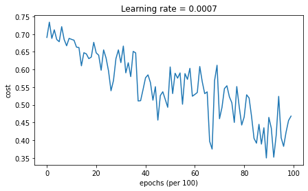
Accuracy: 0.7966666666666666

【HW】L2W2-梯度下降的优化 - 图67

5.2 带冲量的小批量梯度下降

运行以下代码，以查看模型如何使用冲量。因为此示例相对简单，所以使用冲量的收益很小。但是对于更复杂的问题，你可能会看到更大的收获。

# train 3-layer model
layers_dims = [train_X.shape[0], 5, 2, 1]
parameters = model(train_X, train_Y, layers_dims, beta = 0.9, optimizer = "momentum")
# Predict
predictions = predict(train_X, train_Y, parameters)
# Plot decision boundary
plt.title("Model with Momentum optimization")
axes = plt.gca()
axes.set_xlim([-1.5,2.5])
axes.set_ylim([-1,1.5])
plot_decision_boundary(lambda x: predict_dec(parameters, x.T), train_X, train_Y)

Cost after epoch 0: 0.690741
Cost after epoch 1000: 0.685341
Cost after epoch 2000: 0.647145
Cost after epoch 3000: 0.619594
Cost after epoch 4000: 0.576665
Cost after epoch 5000: 0.607324
Cost after epoch 6000: 0.529476
Cost after epoch 7000: 0.460936
Cost after epoch 8000: 0.465780
Cost after epoch 9000: 0.464740

【HW】L2W2-梯度下降的优化 - 图68

Accuracy: 0.7966666666666666

【HW】L2W2-梯度下降的优化 - 图69

5.3 Adam模式的小批量梯度下降

运行以下代码以查看使用Adam的模型表现

# train 3-layer model
layers_dims = [train_X.shape[0], 5, 2, 1]
parameters = model(train_X, train_Y, layers_dims, optimizer = "adam")
# Predict
predictions = predict(train_X, train_Y, parameters)
# Plot decision boundary
plt.title("Model with Adam optimization")
axes = plt.gca()
axes.set_xlim([-1.5,2.5])
axes.set_ylim([-1,1.5])
plot_decision_boundary(lambda x: predict_dec(parameters, x.T), train_X, train_Y)

Cost after epoch 0: 0.690552
Cost after epoch 1000: 0.185501
Cost after epoch 2000: 0.150830
Cost after epoch 3000: 0.074454
Cost after epoch 4000: 0.125959
Cost after epoch 5000: 0.104344
Cost after epoch 6000: 0.100676
Cost after epoch 7000: 0.031652
Cost after epoch 8000: 0.111973
Cost after epoch 9000: 0.197940

【HW】L2W2-梯度下降的优化 - 图70

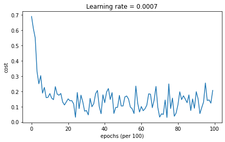
Accuracy: 0.94

【HW】L2W2-梯度下降的优化 - 图71

5.4 总结

优化方法	准确度	模型损失
Gradient descent	79.70％	振荡
Momentum	79.70％	振荡
Adam	94％	更光滑

冲量通常会有所帮助，但是鉴于学习率低和数据集过于简单，其影响几乎可以忽略不计。同样，你看到损失的巨大波动是因为对于优化算法，某些小批处理比其他小批处理更为困难。

另一方面，Adam明显胜过小批次梯度下降和冲量。如果你在此简单数据集上运行更多epoch，则这三种方法都将产生非常好的结果。但是，Adam收敛得更快。

Adam的优势包括：

相对较低的内存要求（尽管高于梯度下降和带冲量的梯度下降）
即使很少调整超参数，通常也能很好地工作（ $【HW】L2W2-梯度下降的优化 - 图72$ 除外）

参考：

Adam paper: https://arxiv.org/pdf/1412.6980.pdf