3-1,低阶API示范
下面的范例使用TensorFlow的低阶API实现线性回归模型和DNN二分类模型。
低阶API主要包括张量操作,计算图和自动微分。
import tensorflow as tf#打印时间分割线@tf.functiondef printbar():today_ts = tf.timestamp()%(24*60*60)hour = tf.cast(today_ts//3600+8,tf.int32)%tf.constant(24)minite = tf.cast((today_ts%3600)//60,tf.int32)second = tf.cast(tf.floor(today_ts%60),tf.int32)def timeformat(m):if tf.strings.length(tf.strings.format("{}",m))==1:return(tf.strings.format("0{}",m))else:return(tf.strings.format("{}",m))timestring = tf.strings.join([timeformat(hour),timeformat(minite),timeformat(second)],separator = ":")tf.print("=========="*8+timestring)
一,线性回归模型
1,准备数据
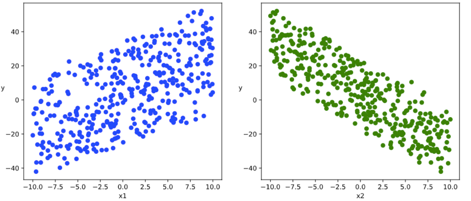
import numpy as npimport pandas as pdfrom matplotlib import pyplot as pltimport tensorflow as tf#样本数量n = 400# 生成测试用数据集X = tf.random.uniform([n,2],minval=-10,maxval=10)w0 = tf.constant([[2.0],[-3.0]])b0 = tf.constant([[3.0]])Y = X@w0 + b0 + tf.random.normal([n,1],mean = 0.0,stddev= 2.0) # @表示矩阵乘法,增加正态扰动
# 数据可视化%matplotlib inline%config InlineBackend.figure_format = 'svg'plt.figure(figsize = (12,5))ax1 = plt.subplot(121)ax1.scatter(X[:,0],Y[:,0], c = "b")plt.xlabel("x1")plt.ylabel("y",rotation = 0)ax2 = plt.subplot(122)ax2.scatter(X[:,1],Y[:,0], c = "g")plt.xlabel("x2")plt.ylabel("y",rotation = 0)plt.show()
# 构建数据管道迭代器def data_iter(features, labels, batch_size=8):num_examples = len(features)indices = list(range(num_examples))np.random.shuffle(indices) #样本的读取顺序是随机的for i in range(0, num_examples, batch_size):indexs = indices[i: min(i + batch_size, num_examples)]yield tf.gather(features,indexs), tf.gather(labels,indexs)# 测试数据管道效果batch_size = 8(features,labels) = next(data_iter(X,Y,batch_size))print(features)print(labels)
tf.Tensor([[ 2.6161194 0.11071014][ 9.79207 -0.70180416][ 9.792343 6.9149055 ][-2.4186516 -9.375019 ][ 9.83749 -3.4637213 ][ 7.3953056 4.374569 ][-0.14686584 -0.28063297][ 0.49001217 -9.739792 ]], shape=(8, 2), dtype=float32)tf.Tensor([[ 9.334667 ][22.058844 ][ 3.0695205][26.736238 ][35.292133 ][ 4.2943544][ 1.6713585][34.826904 ]], shape=(8, 1), dtype=float32)
2,定义模型
w = tf.Variable(tf.random.normal(w0.shape))b = tf.Variable(tf.zeros_like(b0,dtype = tf.float32))# 定义模型class LinearRegression:#正向传播def __call__(self,x):return x@w + b# 损失函数def loss_func(self,y_true,y_pred):return tf.reduce_mean((y_true - y_pred)**2/2)model = LinearRegression()
3,训练模型
# 使用动态图调试def train_step(model, features, labels):with tf.GradientTape() as tape:predictions = model(features)loss = model.loss_func(labels, predictions)# 反向传播求梯度dloss_dw,dloss_db = tape.gradient(loss,[w,b])# 梯度下降法更新参数w.assign(w - 0.001*dloss_dw)b.assign(b - 0.001*dloss_db)return loss
# 测试train_step效果batch_size = 10(features,labels) = next(data_iter(X,Y,batch_size))train_step(model,features,labels)
<tf.Tensor: shape=(), dtype=float32, numpy=211.09982>
def train_model(model,epochs):for epoch in tf.range(1,epochs+1):for features, labels in data_iter(X,Y,10):loss = train_step(model,features,labels)if epoch%50==0:printbar()tf.print("epoch =",epoch,"loss = ",loss)tf.print("w =",w)tf.print("b =",b)train_model(model,epochs = 200)
================================================================================16:35:56epoch = 50 loss = 1.78806472w = [[1.97554708][-2.97719598]]b = [[2.60692883]]================================================================================16:36:00epoch = 100 loss = 2.64588404w = [[1.97319281][-2.97810626]]b = [[2.95525956]]================================================================================16:36:04epoch = 150 loss = 1.42576694w = [[1.96466208][-2.98337793]]b = [[3.00264144]]================================================================================16:36:08epoch = 200 loss = 1.68992615w = [[1.97718477][-2.983814]]b = [[3.01013041]]
##使用autograph机制转换成静态图加速@tf.functiondef train_step(model, features, labels):with tf.GradientTape() as tape:predictions = model(features)loss = model.loss_func(labels, predictions)# 反向传播求梯度dloss_dw,dloss_db = tape.gradient(loss,[w,b])# 梯度下降法更新参数w.assign(w - 0.001*dloss_dw)b.assign(b - 0.001*dloss_db)return lossdef train_model(model,epochs):for epoch in tf.range(1,epochs+1):for features, labels in data_iter(X,Y,10):loss = train_step(model,features,labels)if epoch%50==0:printbar()tf.print("epoch =",epoch,"loss = ",loss)tf.print("w =",w)tf.print("b =",b)train_model(model,epochs = 200)
================================================================================16:36:35epoch = 50 loss = 0.894210339w = [[1.96927285][-2.98914337]]b = [[3.00987792]]================================================================================16:36:36epoch = 100 loss = 1.58621466w = [[1.97566223][-2.98550248]]b = [[3.00998402]]================================================================================16:36:37epoch = 150 loss = 2.2695992w = [[1.96664226][-2.99248481]]b = [[3.01028705]]================================================================================16:36:38epoch = 200 loss = 1.90848124w = [[1.98000824][-2.98888135]]b = [[3.01085401]]
# 结果可视化%matplotlib inline%config InlineBackend.figure_format = 'svg'plt.figure(figsize = (12,5))ax1 = plt.subplot(121)ax1.scatter(X[:,0],Y[:,0], c = "b",label = "samples")ax1.plot(X[:,0],w[0]*X[:,0]+b[0],"-r",linewidth = 5.0,label = "model")ax1.legend()plt.xlabel("x1")plt.ylabel("y",rotation = 0)ax2 = plt.subplot(122)ax2.scatter(X[:,1],Y[:,0], c = "g",label = "samples")ax2.plot(X[:,1],w[1]*X[:,1]+b[0],"-r",linewidth = 5.0,label = "model")ax2.legend()plt.xlabel("x2")plt.ylabel("y",rotation = 0)plt.show()

二,DNN二分类模型
1,准备数据
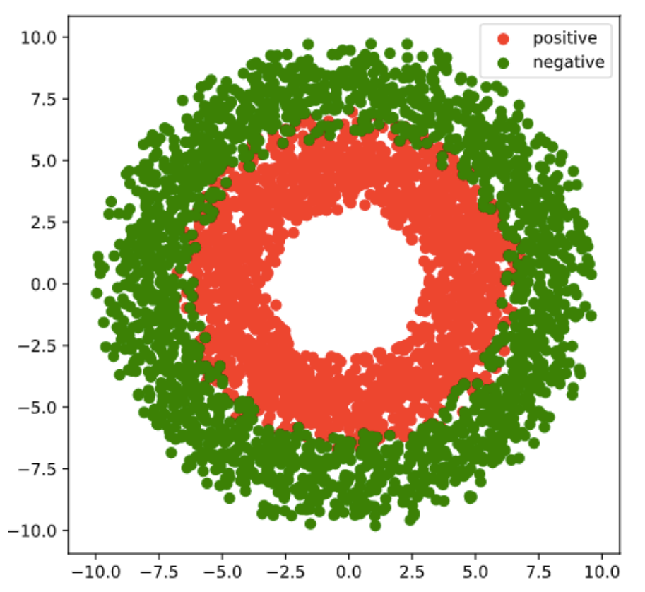
import numpy as npimport pandas as pdfrom matplotlib import pyplot as pltimport tensorflow as tf%matplotlib inline%config InlineBackend.figure_format = 'svg'#正负样本数量n_positive,n_negative = 2000,2000#生成正样本, 小圆环分布r_p = 5.0 + tf.random.truncated_normal([n_positive,1],0.0,1.0)theta_p = tf.random.uniform([n_positive,1],0.0,2*np.pi)Xp = tf.concat([r_p*tf.cos(theta_p),r_p*tf.sin(theta_p)],axis = 1)Yp = tf.ones_like(r_p)#生成负样本, 大圆环分布r_n = 8.0 + tf.random.truncated_normal([n_negative,1],0.0,1.0)theta_n = tf.random.uniform([n_negative,1],0.0,2*np.pi)Xn = tf.concat([r_n*tf.cos(theta_n),r_n*tf.sin(theta_n)],axis = 1)Yn = tf.zeros_like(r_n)#汇总样本X = tf.concat([Xp,Xn],axis = 0)Y = tf.concat([Yp,Yn],axis = 0)#可视化plt.figure(figsize = (6,6))plt.scatter(Xp[:,0].numpy(),Xp[:,1].numpy(),c = "r")plt.scatter(Xn[:,0].numpy(),Xn[:,1].numpy(),c = "g")plt.legend(["positive","negative"]);
# 构建数据管道迭代器def data_iter(features, labels, batch_size=8):num_examples = len(features)indices = list(range(num_examples))np.random.shuffle(indices) #样本的读取顺序是随机的for i in range(0, num_examples, batch_size):indexs = indices[i: min(i + batch_size, num_examples)]yield tf.gather(features,indexs), tf.gather(labels,indexs)# 测试数据管道效果batch_size = 10(features,labels) = next(data_iter(X,Y,batch_size))print(features)print(labels)
tf.Tensor([[ 0.03732629 3.5783494 ][ 0.542919 5.035079 ][ 5.860281 -2.4476354 ][ 0.63657564 3.194231 ][-3.5072308 2.5578873 ][-2.4109735 -3.6621518 ][ 4.0975413 -2.4172943 ][ 1.9393908 -6.782317 ][-4.7453732 -0.5176727 ][-1.4057113 -7.9775257 ]], shape=(10, 2), dtype=float32)tf.Tensor([[1.][1.][0.][1.][1.][1.][1.][0.][1.][0.]], shape=(10, 1), dtype=float32)
2,定义模型
此处范例我们利用tf.Module来组织模型变量,关于tf.Module的较详细介绍参考本书第四章最后一节: Autograph和tf.Module。
class DNNModel(tf.Module):def __init__(self,name = None):super(DNNModel, self).__init__(name=name)self.w1 = tf.Variable(tf.random.truncated_normal([2,4]),dtype = tf.float32)self.b1 = tf.Variable(tf.zeros([1,4]),dtype = tf.float32)self.w2 = tf.Variable(tf.random.truncated_normal([4,8]),dtype = tf.float32)self.b2 = tf.Variable(tf.zeros([1,8]),dtype = tf.float32)self.w3 = tf.Variable(tf.random.truncated_normal([8,1]),dtype = tf.float32)self.b3 = tf.Variable(tf.zeros([1,1]),dtype = tf.float32)# 正向传播@tf.function(input_signature=[tf.TensorSpec(shape = [None,2], dtype = tf.float32)])def __call__(self,x):x = tf.nn.relu(x@self.w1 + self.b1)x = tf.nn.relu(x@self.w2 + self.b2)y = tf.nn.sigmoid(x@self.w3 + self.b3)return y# 损失函数(二元交叉熵)@tf.function(input_signature=[tf.TensorSpec(shape = [None,1], dtype = tf.float32),tf.TensorSpec(shape = [None,1], dtype = tf.float32)])def loss_func(self,y_true,y_pred):#将预测值限制在 1e-7 以上, 1 - 1e-7 以下,避免log(0)错误eps = 1e-7y_pred = tf.clip_by_value(y_pred,eps,1.0-eps)bce = - y_true*tf.math.log(y_pred) - (1-y_true)*tf.math.log(1-y_pred)return tf.reduce_mean(bce)# 评估指标(准确率)@tf.function(input_signature=[tf.TensorSpec(shape = [None,1], dtype = tf.float32),tf.TensorSpec(shape = [None,1], dtype = tf.float32)])def metric_func(self,y_true,y_pred):y_pred = tf.where(y_pred>0.5,tf.ones_like(y_pred,dtype = tf.float32),tf.zeros_like(y_pred,dtype = tf.float32))acc = tf.reduce_mean(1-tf.abs(y_true-y_pred))return accmodel = DNNModel()
# 测试模型结构batch_size = 10(features,labels) = next(data_iter(X,Y,batch_size))predictions = model(features)loss = model.loss_func(labels,predictions)metric = model.metric_func(labels,predictions)tf.print("init loss:",loss)tf.print("init metric",metric)
init loss: 1.76568353init metric 0.6
print(len(model.trainable_variables))
6
3,训练模型
##使用autograph机制转换成静态图加速@tf.functiondef train_step(model, features, labels):# 正向传播求损失with tf.GradientTape() as tape:predictions = model(features)loss = model.loss_func(labels, predictions)# 反向传播求梯度grads = tape.gradient(loss, model.trainable_variables)# 执行梯度下降for p, dloss_dp in zip(model.trainable_variables,grads):p.assign(p - 0.001*dloss_dp)# 计算评估指标metric = model.metric_func(labels,predictions)return loss, metricdef train_model(model,epochs):for epoch in tf.range(1,epochs+1):for features, labels in data_iter(X,Y,100):loss,metric = train_step(model,features,labels)if epoch%100==0:printbar()tf.print("epoch =",epoch,"loss = ",loss, "accuracy = ", metric)train_model(model,epochs = 600)
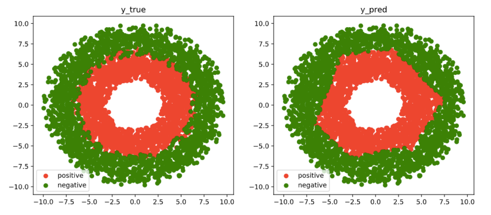
================================================================================16:47:35epoch = 100 loss = 0.567795336 accuracy = 0.71================================================================================16:47:39epoch = 200 loss = 0.50955683 accuracy = 0.77================================================================================16:47:43epoch = 300 loss = 0.421476126 accuracy = 0.84================================================================================16:47:47epoch = 400 loss = 0.330618203 accuracy = 0.9================================================================================16:47:51epoch = 500 loss = 0.308296859 accuracy = 0.89================================================================================16:47:55epoch = 600 loss = 0.279367268 accuracy = 0.96
# 结果可视化fig, (ax1,ax2) = plt.subplots(nrows=1,ncols=2,figsize = (12,5))ax1.scatter(Xp[:,0],Xp[:,1],c = "r")ax1.scatter(Xn[:,0],Xn[:,1],c = "g")ax1.legend(["positive","negative"]);ax1.set_title("y_true");Xp_pred = tf.boolean_mask(X,tf.squeeze(model(X)>=0.5),axis = 0)Xn_pred = tf.boolean_mask(X,tf.squeeze(model(X)<0.5),axis = 0)ax2.scatter(Xp_pred[:,0],Xp_pred[:,1],c = "r")ax2.scatter(Xn_pred[:,0],Xn_pred[:,1],c = "g")ax2.legend(["positive","negative"]);ax2.set_title("y_pred");

若有收获,就点个赞吧
0 人点赞
