• Bayes theorem
• Naïve Bayes algorithm
• Evaluating ML models
• Evaluation procedures
• Holdout method
• Cross validation
• Leave-one-out cross validation
• Cross-validation for parameter tuning
• Performance measures
• Accuracy, recall, precision and F1 score; confusion matrix
Probabilistic classification method computes the class probability .
Naive Bayes is a prominent example of this group.
后验概率也叫条件概率 posteriori probability 
prior probability
贝叶斯公式解决分类问题的两个假设:
1)Independence - (the values of the) attributes are conditionally independent of each other, given the class (i.e. for each class value)
2)Equally importance – all attributes are equally important
不现实的假设,几乎永不正确;但是这些简单的假设导致算法容易实现,而且效果良好。
Example: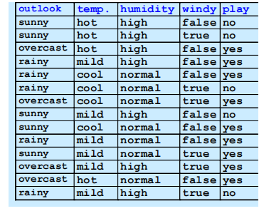
E1 = outlook=sunny, E2 = temperature=cool
E3 = humidity=high, E4 = windy=true (条件是预测时给定的)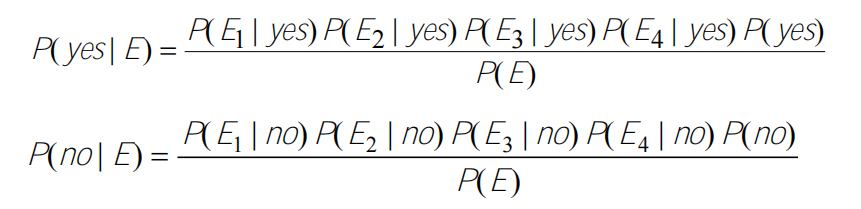
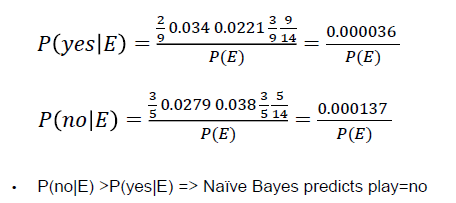
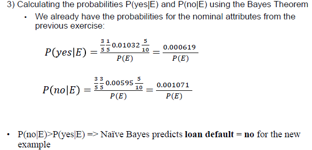
• Top parts: the probabilities will be calculated from the training data
• Bottom parts: P(E) in both cases - the same for class yes and no. Since we take the decision by comparing P(yes|E) and P(yes|no), there is no need to calculate P(E), we will just compare the top parts.
“Zero frequency” problem
如果有一个属性和类别总是同时出现,其他属性就不起作用了
补救措施就是laplace correction
分类时:朴素贝叶斯很容易处理缺失属性,因为各属性独立,所以缺失属性的后验概率不出现在公式中即可。
训练时:不在计数中包括缺失值,根据实际训练示例数量计算每个属性缺失值的概率。
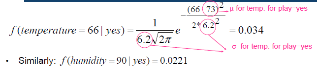
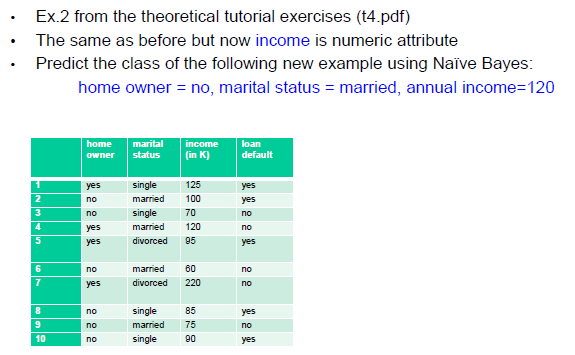
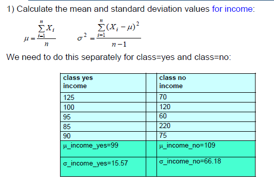
朴素贝叶斯用于数值属性
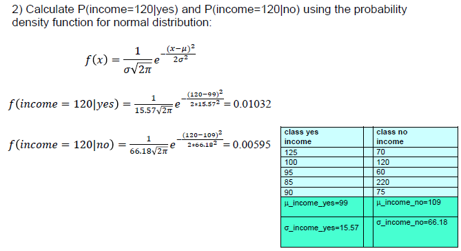
假设数值属性遵循正态分布(Gaussian Distribution)和 probability density function.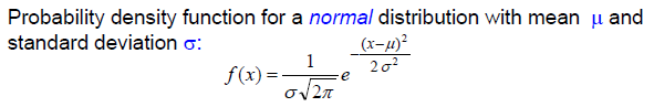
The probability density function is not exactly the probability but it is closely
related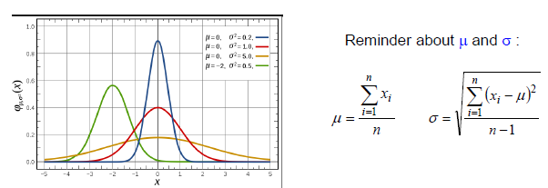
对每一个数值数值属性,分割每个类别的值,计算μ和σ(对于每个属性-类的组合)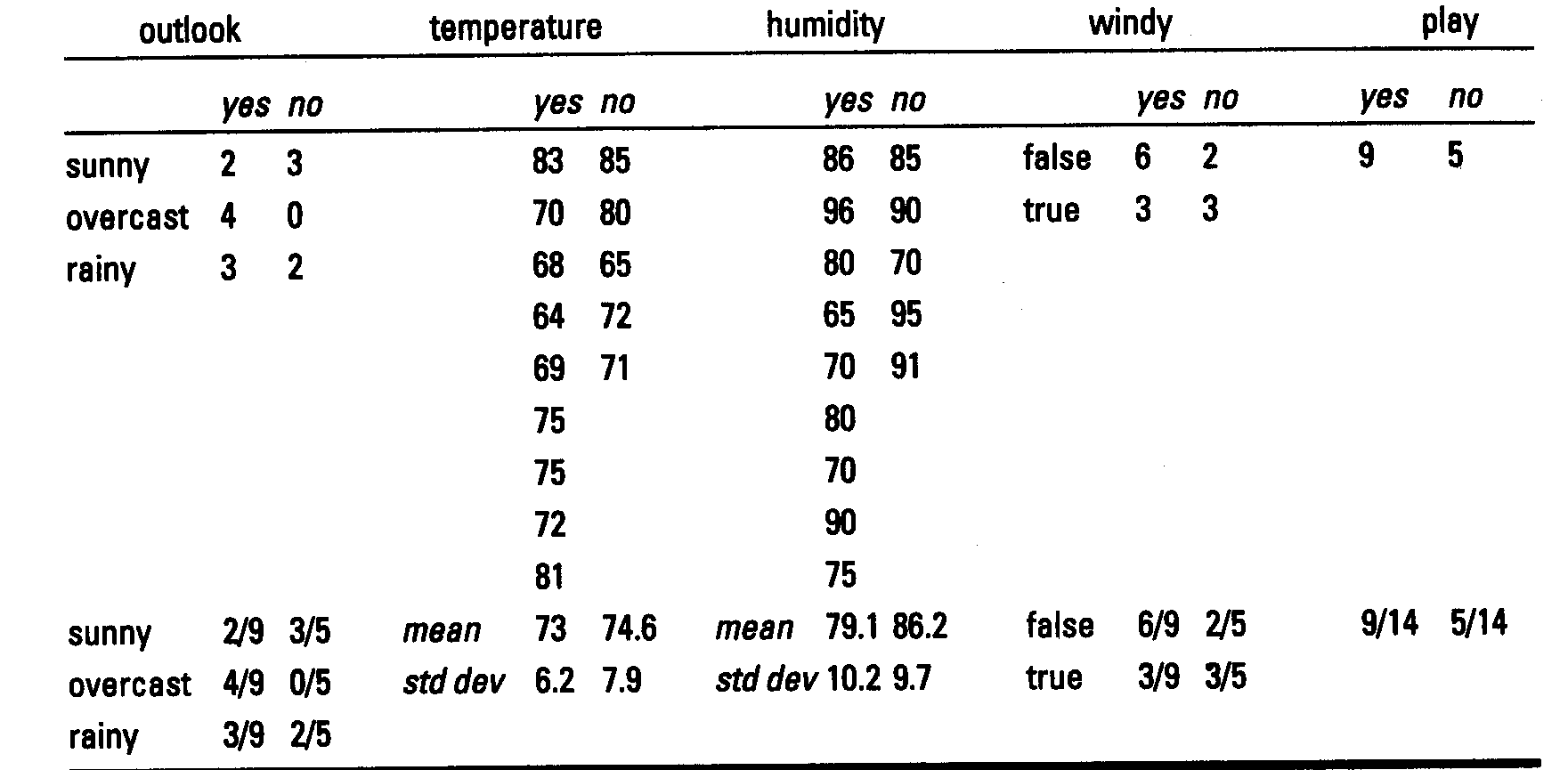
- 由于独立假设,概率的计算很容易
- 快速—只需扫描一次训练数据就能计算出所有的统计数据,包括名义属性和连续属性。
名义和连续属性的所有统计数据 - 在许多情况下优于更复杂的学习方法
- 对孤立的噪声点具有鲁棒性—这些噪声点对条件概率的影响可忽略不计
对条件概率的影响可以忽略不计 - 相关的属性降低了奈何贝叶斯的能力—违反了独立假设。
独立假设- 解决方案:事先应用特征选择,以识别和抛弃
相关的(多余的)属性
- 解决方案:事先应用特征选择,以识别和抛弃
- 数字属性的正态分布假设—许多特征
不是正态分布 - 解决方案。 - 首先将数据具体化,即数字->名义属性
- 使用其他概率密度函数,例如泊松、二项、伽马
• Probabilities are calculated easily due to the independence assumption
• Fast - requires 1 scan of the training data to calculate all statistics for
both nominal and continuous attributes
• In many cases outperforms more sophisticated learning methods
• Robust to isolated noise points – such points have only negligible impact
on the conditional probabilities
• Correlated attributes reduce the power of Naïve Bayes - violation of the
independence assumption
• Solution: apply feature selection beforehand to identify and discard
correlated (redundant) attributes
• Normal distribution assumption for numeric attributes - many features
are not normally distributed – solutions:
• Discretize the data first, i.e. numerical -> nominal attributes
• Use other probability density functions, e.g. Poisson, binomial, gamma
Evaluating Machine Learning Algorithms
Evaluation Procedures
• Holdout method(搁置法)
随机分,训练集2/3->建模, 测试集1/3->评估模型(准确率或者其他性能衡量)
ACC = 正确分类的个数/预测结果的总个数
训练集的ACC过于乐观,不是一个好的泛化性能的指标
• Cross validation
有时候需要validation set, 把数据集分为 training, validation和test, 例如:决策树,神经网络运行在两个阶段:
1. 建立分类器1. 优化超参
测试集不能用于优化超参
超参数 - 可以调整的参数,以优化ML算法的性能。与作为模型一部分的基本参数不同,如线性回归模型中的系数。比如:kmeans聚类中的k;neural network 隐藏层的层数, 训练epoch。在ML中,调参就是优化超参。
由于训练集和测试集的划分是随机的,如果没有分层
训练集和测试集中可能缺少某些类别,或者是代表性不足,例如,如果训练集中缺少某个类别的所有例子
他们去了测试集),分类器就不能学会预测这个类别。因此分层可以解决这个问题,同时分层可以和holdout 方法一起用->an improved holdout method
确保每个类别在两个数据集(训练和测试)中的代表比例大致相同。例如,如果整个数据集中的类别比例是60%的Class1和40
% Class2,这个比例在训练和测试部分保持不变。
重复搁置法 可以通过以下方式变得更加可靠
训练集和测试集的随机拆分几次,并计算出
平均精度.
  - 例如,重复10次:在这10次运行中的每一次,都随机选择一定比例(例如<br />2/3)被随机选择用于训练(可能有分层),并且提醒用于测试
  - 将10次的准确率平均化,以产生一个总的平均准确率
  - 我们可以做得更好,例如,通过防止测试集之间的重叠。
• Leave-one-out cross validation
防止测试集之间的重叠。
十折交叉验证
第1步:将数据分成10个大小大致相同的集合set1,…, set10
第2步:建立一个分类器10次。每次测试是在1个集合上进行的(蓝色),训练是在其余9个集合上进行的(白色)。训练是在其余9个集合上进行的(白色)。
Run1: train on set1+…set9, test on set10 and calculate accuracy (acc1)
Run2: train on set1+…set8+set10, test on set9 and calculate accuracy (acc2)
….
Run10: train on set2+…set10, test on set1 and calculate accuracy (acc10)
第3步:计算交叉验证的准确性=平均(acc1,acc2,…acc10)。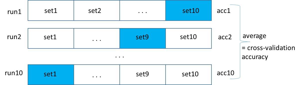
十折交叉验证是标准评估方法, 每一个子集用了分层法。
  - 广泛的实验表明,这是获得准确估计的最佳选择。
  - 也有一些理论上的证据证明了这一点
  - **_重复分层的10倍交叉验证法_**甚至更好- 例如,10倍交叉验证重复10次,结果取平均值。减少了分割数据的差异性
• Cross-validation for parameter tuning
- N折交叉验证的一种特殊形式
- 将褶皱(fold)的数量设定为训练实例的数量
- =>对于n个训练实例,建立分类器n次
- 优点
- 最有效地利用了数据—尽可能多的数据被用于训练
- 确定性的程序—不涉及随机抽样—每次都得到相同的结果
- 劣势
- 计算成本高,特别是对大数据集而言
- 我们还可以使用交叉验证法来搜索不同的参数组合,并选择最好的一个
- 让我们考虑k-Nearest Neighbor和它的两个参数—k和distance测量类型;我们可以通过以下组合进行搜索。
- 最近的邻居数k=1、3、5、11和13
- 距离测量—曼哈顿和欧几里得
- => 5 x 2的参数值组合
- 我们希望找到最好的组合—能够很好地概括新的例子的组合。
- 我们将使用以下程序,称为交叉验证的网格搜索来调整参数
- 创建参数网格(即参数组合)。将数据分成训练集和测试集
- 让我们考虑k-Nearest Neighbor和它的两个参数—k和distance测量类型;我们可以通过以下组合进行搜索。
对于每个参数组合
使用10倍交叉验证法在训练数据上训练一个k-NN分类器
计算交叉验证的准确性cv_acc
如果cv_acc > best_cv_acc
best_cv_acc = cv_acc
best_parameters = 当前参数
使用整个训练数据和best_parameters重新建立k-NN模型
在测试数据上进行评估并报告结果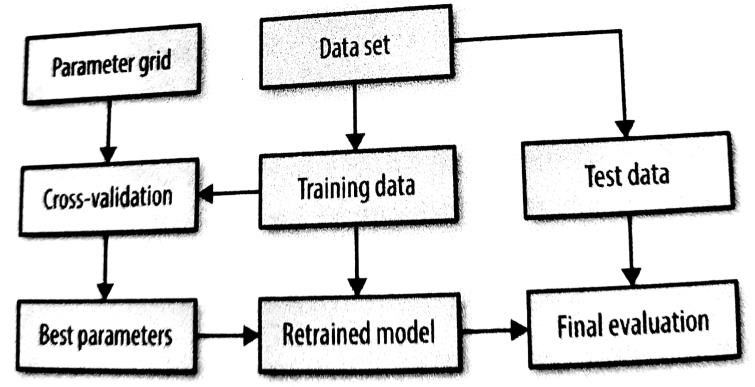
     - 数据被分割成训练集和测试集
     - 交叉验证循环使用训练数据
        - 对每个参数组合都进行交叉验证
        - 其目的是选择最佳参数组合--具有最高交叉验证准确性的参数组合
        - 这涉及到,对于每个参数组合,在90%的训练数据上建立10个模型(9个折),并在剩下的10%(1个折)上对它们进行评估。
     - 一旦完成,在整个训练集上使用选定的最佳参数组合训练一个新的模型,并在测试集上进行评估。
     - 在sklearn中,我们可以使用GridSearchCV来做到这一点--参见教程中的练习,使用<br />练习:Python
More Performance Measures
• Confusion matrix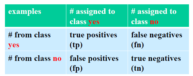
accuracy= (tp+tn)/(tp+fn+fp+tn) 对角线上值的和/矩阵中所有值的和
混淆矩阵不是一个绩效衡量标准,它允许我们计算绩效衡量标准。
• Recall, precision and F1 score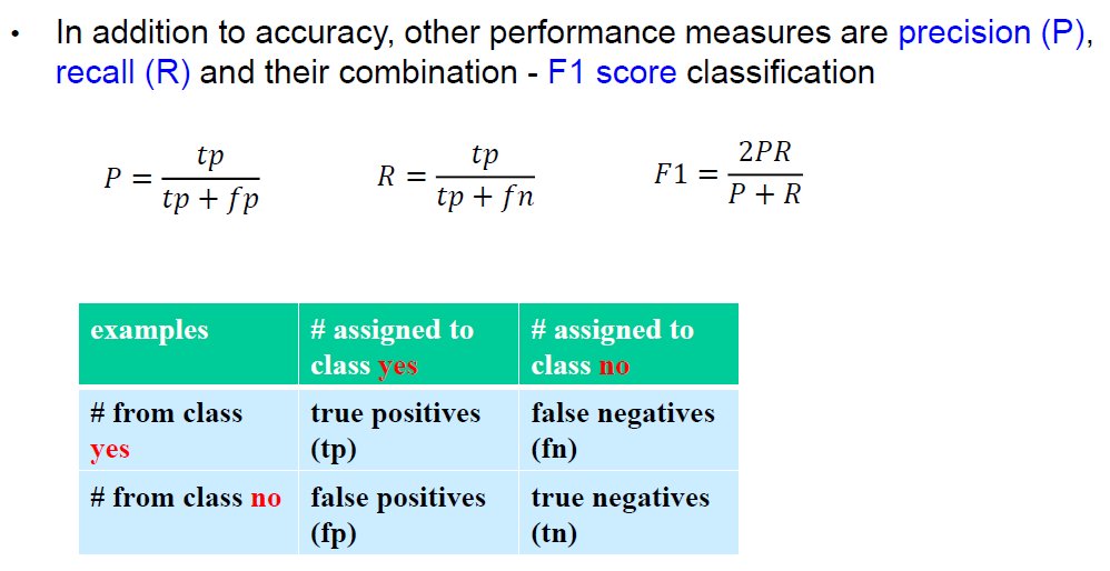

若有收获,就点个赞吧
0 人点赞
