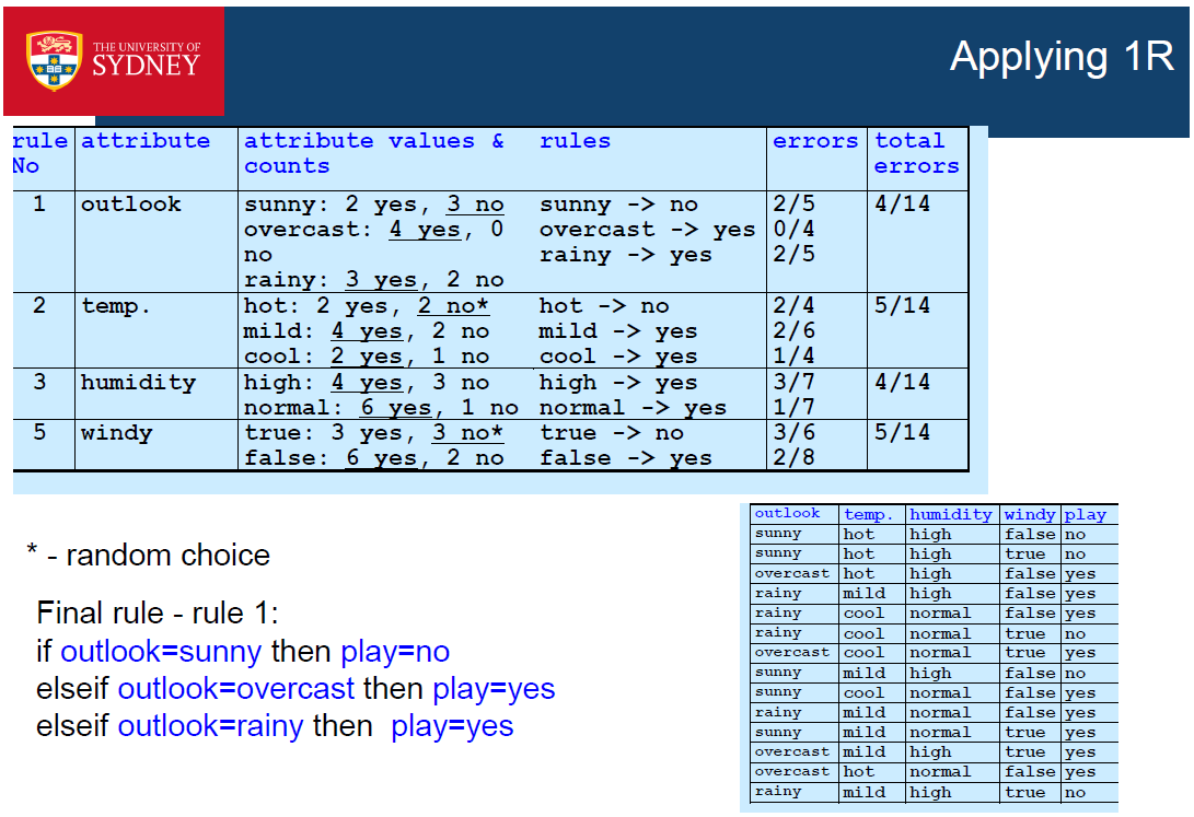
Nearest Neighbor Algorithm
| a1 | a2 | a3 | class | |
|---|---|---|---|---|
| 1 | 1 | 3 | 1 | yes |
| 2 | 3 | 5 | 2 | yes |
| 3 | 3 | 2 | 2 | no |
| 4 | 5 | 2 | 3 | no |
What will be the prediction of the Nearest Neighbor algorithm using the Euclidean distance for the following new example: a1=2, a2=4, a3=2?
Ans:
D(new, ex1) =  =
=  Yes
Yes
D(new, ex2) =  =
=  Yes
Yes
D(new, ex3) =  =
=  No
No
D(new, ex4) =  =
=  No
No
∵ D(new, ex2) is the closest.
∴ The result of new example is yes according to 1NN algorithm.
Computational complexity
- Training is fast – no model is built; just storing training examples
- Classification (prediction for a new example)
- Compare each unseen example with each training example
- If m training examples with dimensionality n => lookup for 1 unseen example takes m*n computations, i.e. O(mn)
- Memory requirements – you need to remember each training example, O(mn)
- Impractical for large data due to time and memory requirements
- However, there are variations allowing to find the nearest neighbours more efficiently
- e.g. by using more efficient data structures such as KD-trees and ball trees, see Witten p.136-141
KNN
• K-Nearest Neighbor is very sensitive to to the value of k
• rule of thumb: k <= sqrt(#training_examples)
• commercial packages typically use k=10
• Using more nearest neighbors increases the robustness to noisy examples
• K-Nearest Neighbor can be used not only for classification, but also for regression
• The prediction will be the average value of the class values (numerical) of the
k nearest neighbors
Following former example, according to 3NN Algorithm, the 3 nearest neighbors are ex1 (yes), ex2 (yes), and ex3(no); the majority class is yes. ∴3-Nearest Neighbor predicts class =yes
KNN for nominal class, if both are different, the difference of square is 1; otherwise, it is 0.
Weighted nearest neighbor:
Idea: Closer neighbors should count more than distant neighbors.
• Distance-weighted nearest-neighbor algorithm
• Find the k nearest neighbors
• Weight their contribution based on their distance to the new example
• bigger weight if they are closer
• smaller weight if they are further
• e.g. the vote can be weighted according to the disstance – weight
w = 1/d2
Decision boundary of 1-nearest neighbor
• Nearest neighbor classifiers produced decision boundaries with an
arbitrary shape
• The 1-nearest neighbor boundary is formed by the edges of the Voronoi diagram that separate the
points of the two classes
• Voronoi region:
• Each training example has an associated Voronoi region; it contains the
data points for which this is the closest example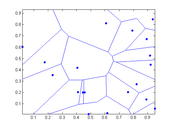
KNN - discussion
• Often very accurate
• Has been used in statistics since 1950s
• Slow for big datasets
• requires efficient data structures such as KD-trees
• Distance-based - requires normalization
• Produces arbitrarily shaped decision boundary defined by a subset of the Voronoi edges
• Not effective for high-dimensional data (data with many features)
• The notion of “nearness” is not effective in high dimensional data
• Solution – dimensionality reduction and feature selection
• Sensitive to the value of k
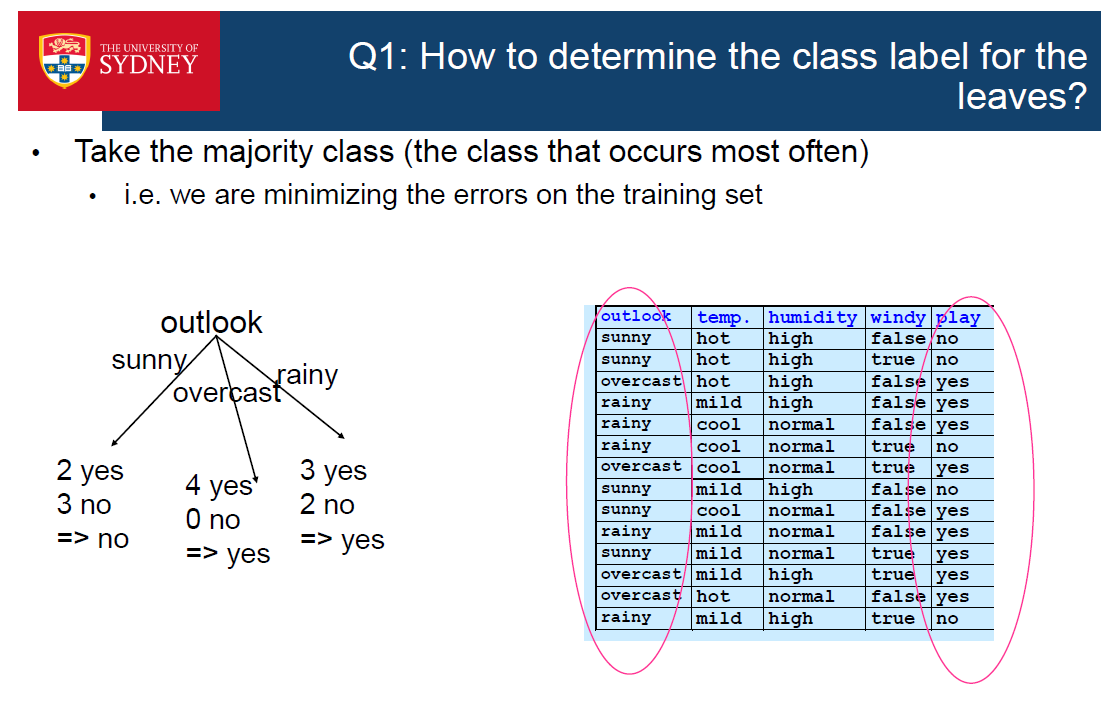
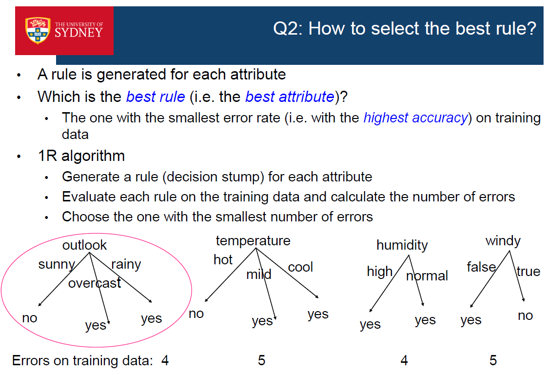
Rule-based Algorithm
- 1R
- 1R stands for “1-rule”
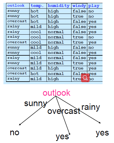
- Generates 1 rule that tests the value of a single attribute
- e.g. a rule that tests the value of outlook
if outlook=sunny then class=no
elseif outlook=overcast then class=yes elseif outlook=rainy then class=yes
- The rule can be represented as a 1-level decision tree
- At the root, test the attribute value
- Each branch correspond to a value
- Each leaf correspond to a class
1R discussion:
• Simple and computationally efficient algorithm
• Produces rules that are easy to understand
• In contrast to “black-box” models such as neural networks
• Sometimes produces surprisingly good results
• It is useful to try the simple algorithms first and compare their performance with more sophisticated algorithms
• Numerical datasets require discretization
• 1R has an in-built procedure to do this
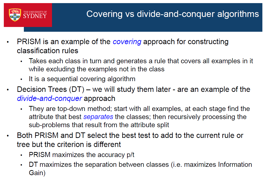
- PRISM (Rule-based Algorithm)
- PRISM is an example of rule-based covering algorithm
- This type of algorithms:
- consider each class in turn and
- construct a set of if-then rules that cover all examples from this class and do not cover any examples from the other classes.
- Called covering algorithms because:
- At each stage of the algorithm, a rule is identified that “covers” some of the examples
- if part of the rules
- contains conditions that test the value of an attribute
- initially empty, tests are added incrementally in order to create a rule with maximum accuracy
if ? then class a
if x1>2 then class a
if x1>2 & x2<5 then class a
if x1>2 & x2<5 & x3<3 then class a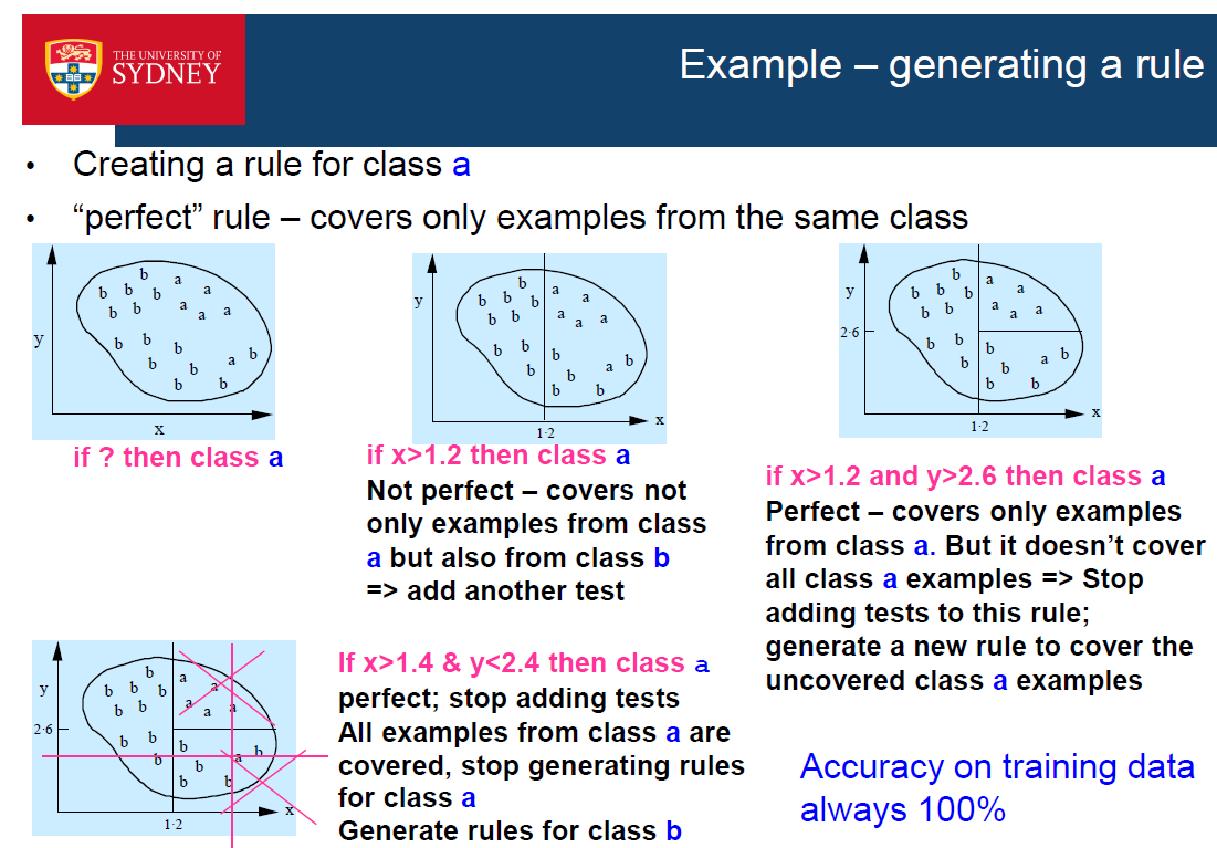
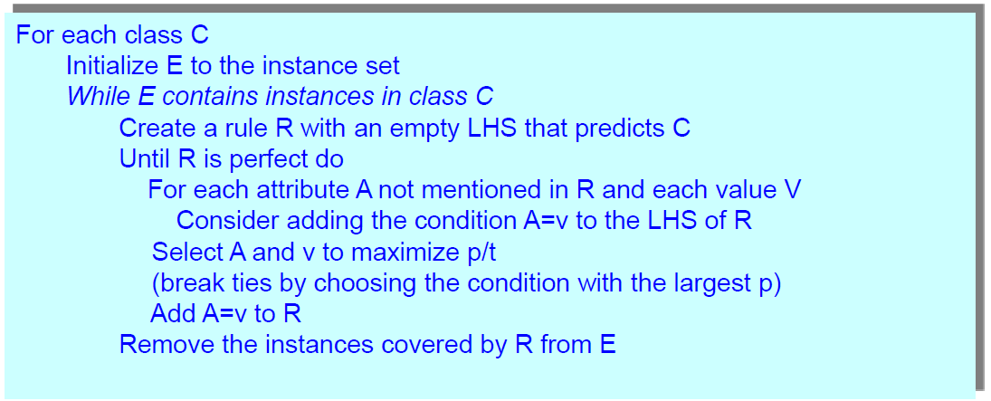
- Idea: Generate a rule by adding tests that maximize the rule’s accuracy
- For each class:
- Start with an empty rule and gradually add conditions
- Each condition tests the value of 1 attribute
- By adding a new test, the rule coverage is reduced (i.e.the rule becomes more specific)
- Finish when p/t=1 (i.e. the rule covers only examples fromthe same class, i.e. is “perfect”)
- Which test to add at each step? The one that maximizes accuracy p/t:
- t: total number of examples (from all classes) covered by the rule (t comes fromtotal)
- p: examples from the class under consideration, covered by the rule (p comesfrom positive)
- t-p: number of errors made by the rule
- Select the test that maximises the accuracy p/t
Example: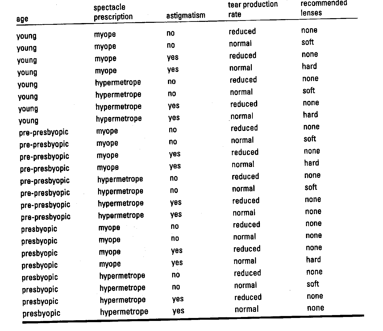
- Start with an empty rule: if ? then recommendation = hard


- Best test (highest accuracy): astigmatism = yes
Note that there is a tie: both astigmatism = yes and tear production rate = normal have the same accuracy 4/12; we choose the first one randomly
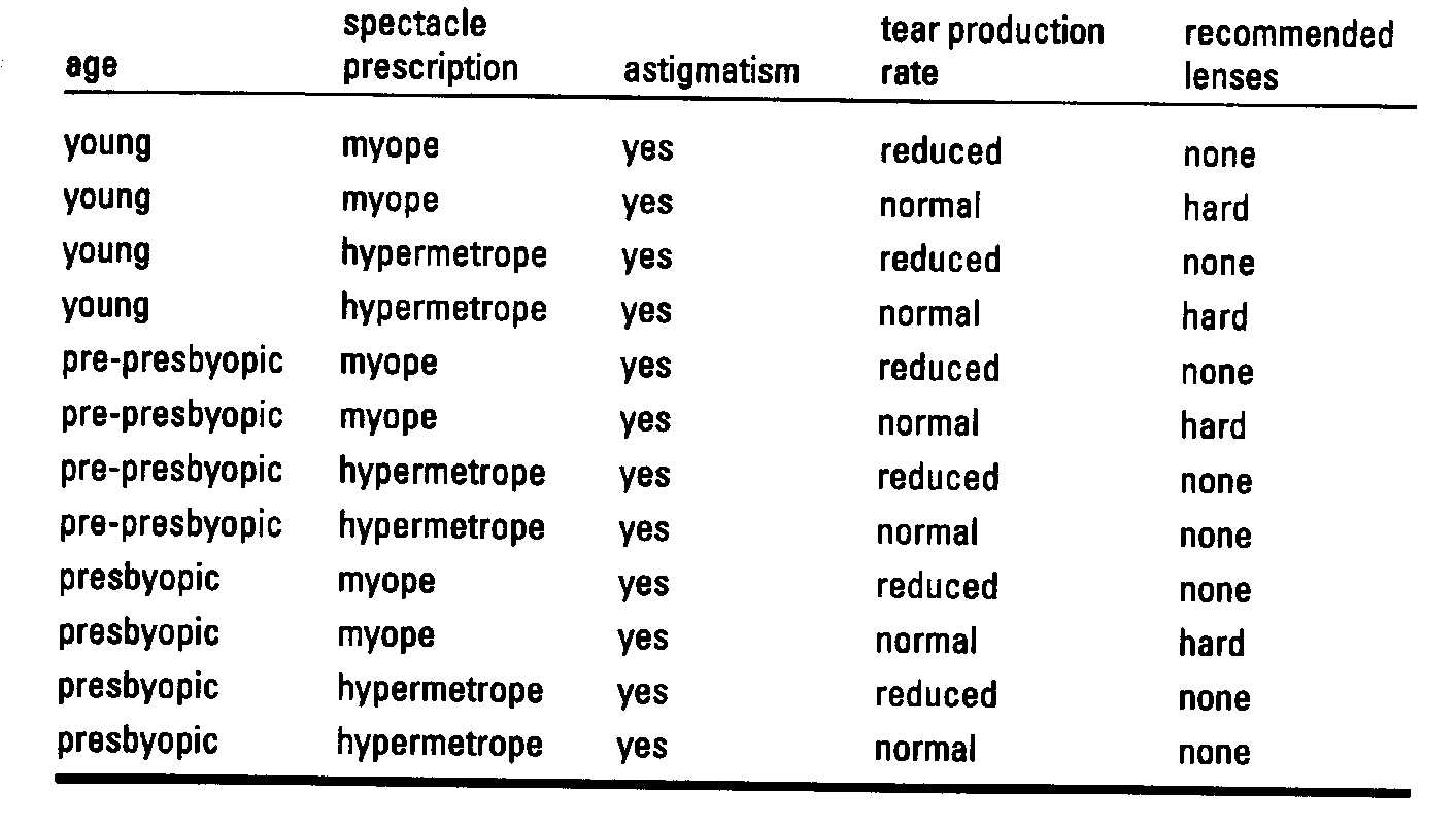
- Current rule: if astigmatism = yes then recommendation = hard
- Not “perfect” - covers 12 examples but only 4 of them are from class hard =>refinement is needed
- Further refinement by adding tests: if astigmatism = yes and ? then recommendation = hard


- Best test: tear production rate = normal
- Current rule: if astigmatism = yes and tear production rate = normal then recommendation = hard
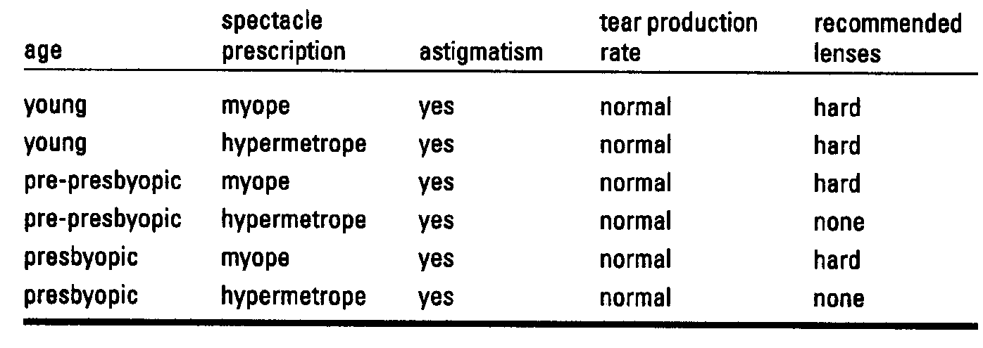
The rule is again not “perfect” – 2 examples classified as none => further refinement is needed
Further refinement: if astigmatism = yes and tear production rate = normal and ? then recommendation = hard


- Best test: tie between the 1st and 4th; choose the one with the greater coverage (4th)
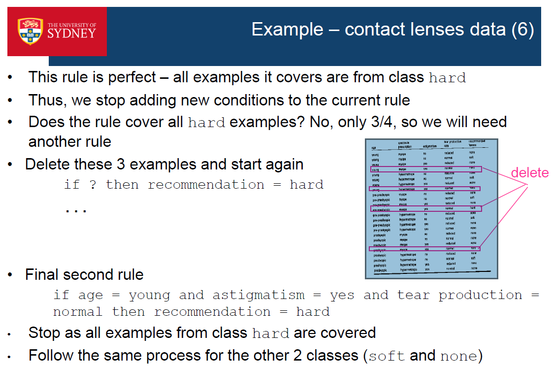
- New rule: if astigmatism = yes & tear production = normal & spectacle prescription = myope then recommendation = hard

若有收获,就点个赞吧
0 人点赞
