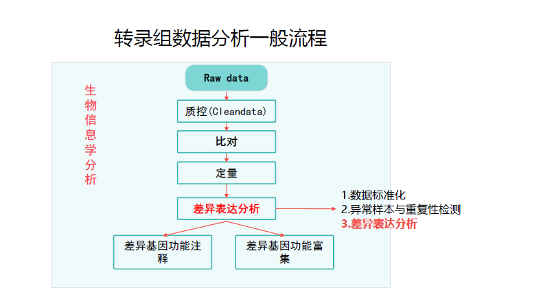
流程

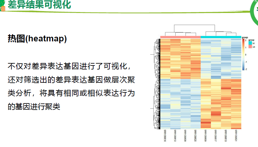
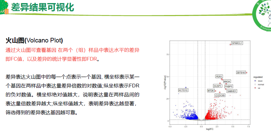
数据分析可视化
本地分析脚本
rm(list = ls())options(stringsAsFactors = F)# 加载包library(edgeR)library(ggplot2)# 读取基因表达矩阵信息并查看分组信息和表达矩阵数据lname <- load(file = "data/Step01-airwayData.Rdata");lname# 表达谱filter_count[1:4,1:4]# 分组信息group_list <- group[match(colnames(filter_count),group$run_accession),2]group_listcomp <- unlist(strsplit("Dex_vs_untreated",split = "_vs_"))group_list <- factor(group_list,levels = comp)group_listtable(group_list)# 构建线性模型。0代表x线性模型的截距为0design <- model.matrix(~0+group_list)rownames(design) <- colnames(filter_count)colnames(design) <- levels(factor(group_list))design# 构建edgeR的DGEList对象DEG <- DGEList(counts=filter_count,group=factor(group_list))# 归一化基因表达分布DEG <- calcNormFactors(DEG)# 计算线性模型的参数DEG <- estimateGLMCommonDisp(DEG,design)DEG <- estimateGLMTrendedDisp(DEG, design)DEG <- estimateGLMTagwiseDisp(DEG, design)# 拟合线性模型fit <- glmFit(DEG, design)# 进行差异分析lrt <- glmLRT(fit, contrast=c(1,-1))# 提取过滤差异分析结果DEG_edgeR <- as.data.frame(topTags(lrt, n=nrow(DEG)))head(DEG_edgeR)# 筛选上下调,设定阈值fc_cutoff <- 1.5pvalue <- 0.05DEG_edgeR$regulated <- "normal"loc_up <- intersect(which( DEG_edgeR$logFC > log2(fc_cutoff) ),which( DEG_edgeR$PValue < pvalue) )loc_down <- intersect(which(DEG_edgeR$logFC < (-log2(fc_cutoff))),which(DEG_edgeR$PValue<pvalue))DEG_edgeR$regulated[loc_up] <- "up"DEG_edgeR$regulated[loc_down] <- "down"table(DEG_edgeR$regulated)## 添加一列gene symbol# 方法1:使用包library(org.Hs.eg.db)keytypes(org.Hs.eg.db)library(clusterProfiler)id2symbol <- bitr(rownames(DEG_edgeR),fromType = "ENSEMBL",toType = "SYMBOL",OrgDb = org.Hs.eg.db)head(id2symbol)DEG_edgeR <- cbind(GeneID=rownames(DEG_edgeR),DEG_edgeR)DEG_edgeR_symbol <- merge(id2symbol,DEG_edgeR,by.x="ENSEMBL",by.y="GeneID",all.y=T)head(DEG_edgeR_symbol)# 方法2:gtf文件中得到的id与name关系# Assembly: GRCh37(hg19) Release: ?# 使用上课测试得到的count做# 选择显著差异表达的结果library(tidyverse)DEG_edgeR_symbol_Sig <- filter(DEG_edgeR_symbol,regulated!="normal")# 保存write.csv(DEG_edgeR_symbol,"result/4.DEG_edgeR_all.csv", row.names = F)write.csv(DEG_edgeR_symbol_Sig,"result/4.DEG_edgeR_Sig.csv", row.names = F)save(DEG_edgeR_symbol,file = "data/Step03-edgeR_nrDEG.Rdata")##====== 检查是否上下调设置错了# 挑选一个差异表达基因head(DEG_edgeR_symbol_Sig)exp <- c(t(express_cpm[match("ENSG00000001626",rownames(express_cpm)),]))test <- data.frame(value=exp, group=group_list)ggplot(data=test,aes(x=group,y=value,fill=group)) + geom_boxplot()
服务器分析传参脚本

原因:
1,可以在服务器上解决数据分析,实现环境统一
2,可以批量跑很多方案
脚本
## 帮助文档
library(getopt)
spec <- matrix(c(
  'help',   'h',  0,  "logical",
  'count',  'c',  1,  "character",
  'group',  'g',  1,  "character",
  'comp',   'C',  1,  "character",
  'fc',     'f',  1,  "numeric",
  'pvalue', 'p',  1,  "numeric",
  'od',     'o',  1,  "character"
), byrow = TRUE, ncol = 4)
opt <- getopt(spec)

print_usage <- function(spec=NULL){
  cat("Usage example: Rscript edgeR.R --count rawdata.txt --group group.txt --od ./
  Options:
    --help  NULL
    --count   character  gene expression , raw count [forced]
    --group   character  group information [forced]
    --comp    character  A vs B, example: Dex_vs_untreated
    --fc      numeric    fold change cutoff, default: 1.5
    --pvalue  numeric    pvalue cutoff, default:0.05
    --od      character  outdir
  \n")
  q(status=1)
}
if (!is.null(opt$help) |is.null(opt$count)  |is.null(opt$od)) { print_usage(spec) }
if (is.null(opt$group) ) { print_usage(spec) }
if (is.null(opt$fc) )    { opt$fc <- 1.5 }
if (is.null(opt$pvalue) ) { opt$pvalue <- 0.05 }
if (!file.exists(opt$od)) { dir.create(opt$od) }

library(edgeR)
library(org.Hs.eg.db)
library(ggplot2)
library(tidyverse)

# 读取基因表达矩阵信息并查看分组信息和表达矩阵数据
# 读取基因表达矩阵
exprSet <- read.delim(opt$count,row.names = 1,sep = "\t",header = T,check.names = F)
# 检查表达谱
dim(exprSet)
exprSet[1:6,1:6]

group <- read.table(opt$group,header = T,sep = "\t",row.names = 1)
head(group)
group <- group[match(rownames(group),colnames(exprSet)),]

# 处理分组信息
comp <- unlist(strsplit(opt$comp,split = "_vs_"))
group_list <- factor(group,levels = comp)
group_list
table(group_list)


# 构建线性模型。0代表x线性模型的截距为0
design <- model.matrix(~0+group_list)
rownames(design) <- colnames(exprSet)
colnames(design) <- comp
design

# 构建edgeR的DGEList对象
DEG <- DGEList(counts=exprSet,  group=factor(group_list))

# 归一化基因表达分布
DEG <- calcNormFactors(DEG)

# 计算线性模型的参数
DEG <- estimateGLMCommonDisp(DEG,design)
DEG <- estimateGLMTrendedDisp(DEG, design)
DEG <- estimateGLMTagwiseDisp(DEG, design)

# 拟合线性模型
fit <- glmFit(DEG, design)

# 进行差异分析,1,-1意味着前比后
lrt <- glmLRT(fit, contrast=c(1,-1))

# 提取过滤差异分析结果
DEG_edgeR <- as.data.frame(topTags(lrt, n=nrow(DEG)))
head(DEG_edgeR)

# 筛选上下调,设定阈值
fc_cutoff <- opt$fc
pvalue <- opt$pvalue

DEG_edgeR$regulated <- "normal"

loc_up <- intersect(which(DEG_edgeR$logFC>log2(fc_cutoff)),
                    which(DEG_edgeR$PValue<pvalue))
loc_down <- intersect(which(DEG_edgeR$logFC < (-log2(fc_cutoff))),
                      which(DEG_edgeR$PValue<pvalue))

DEG_edgeR$regulated[loc_up] <- "up"
DEG_edgeR$regulated[loc_down] <- "down"

table(DEG_edgeR$regulated)

DEG_edgeR <- cbind(GeneID=rownames(DEG_edgeR),DEG_edgeR)
DEG_edgeR_Sig <- filter(DEG_edgeR,regulated!="normal")

# 保存
setwd(opt$od)
write.table(DEG_edgeR,paste0(opt$comp,"_edgeR_all.xls"), row.names = F, sep="\t",quote = F)
write.table(DEG_edgeR_Sig,paste0(opt$comp,"_edgeR_Sig.xls"), row.names = F, sep="\t",quote = F)

若有收获,就点个赞吧
0 人点赞
