Bayesian logistic regression, Generalized linear models (GLMs), Hierarchical models

Lecture 6 - Classification models.pdf

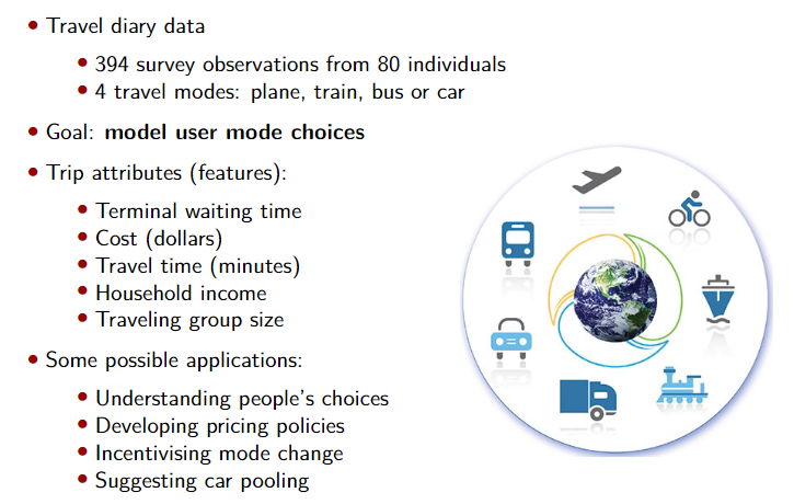
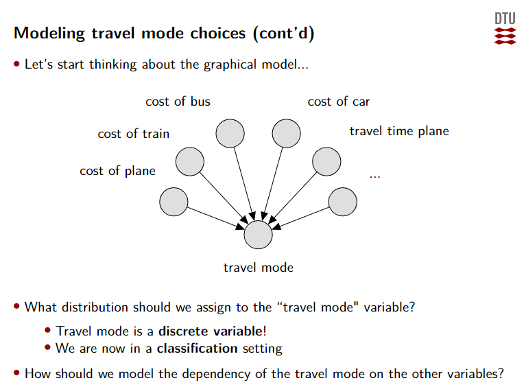
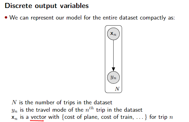
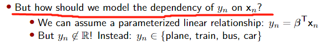
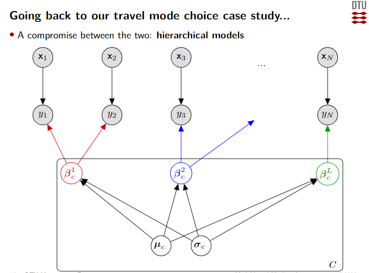
Modeling travel mode choices

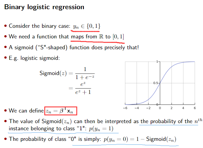
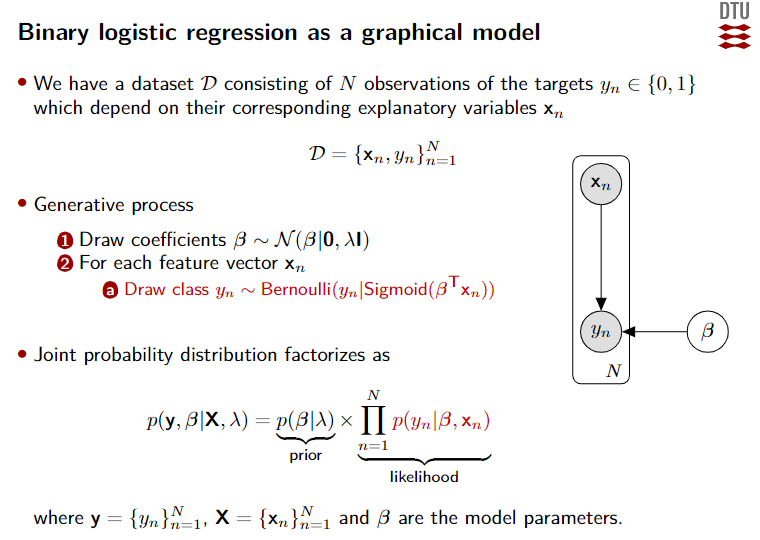
Binary logistic regression

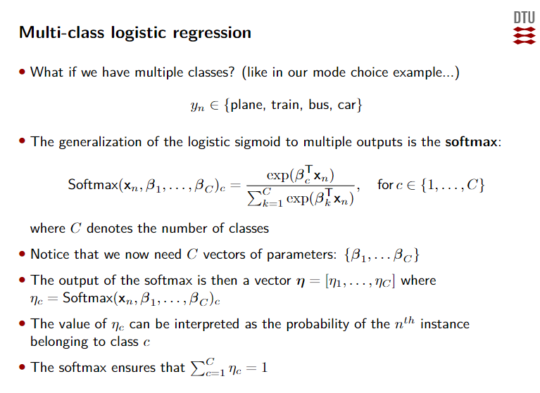
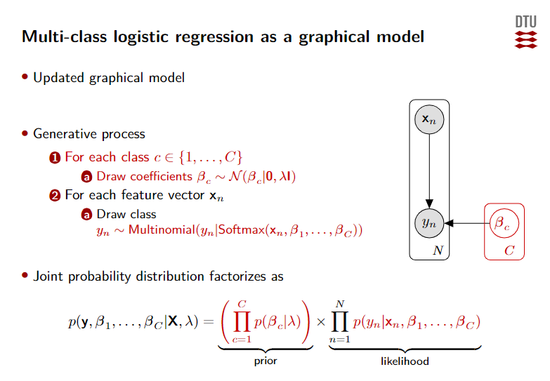
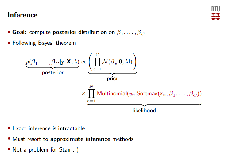
Multi-class logistic regression

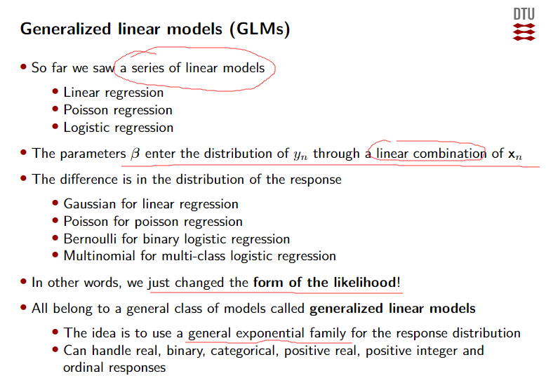
Generalized linear models (GLMs)

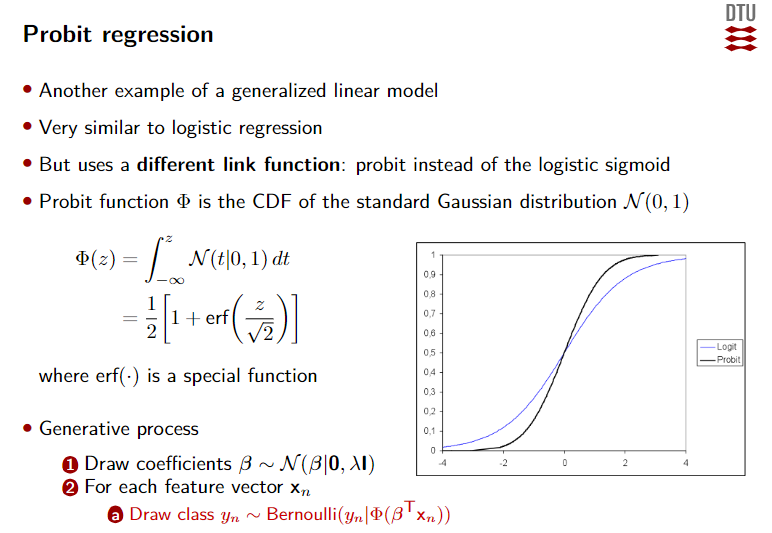
Probit regression

贝叶斯网络的采样

贝叶斯网络的采样 - 知乎

贝叶斯网络，又成为信念网络或有向无环图模型，利用有向无环图来刻画一组随机变量之间的条件概率分布关系。

原始采样法/祖先采样（Ancestral Sampling Approach）

原始采样法是一种针对有向图模型的基础采样方法，指从模型所表示的联合分布中产生样本，又称祖先采样法。该方法所得出的结果即视为原始采样。

作用：对一个没有观测变量的贝叶斯网络进行采样，最简单的方法
核心思想：根据有向图的顺序，先对祖先节点进行采样，只有当某个节点的父节点都已经完成采样，才对该节点进行采样。
按照概率分布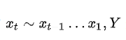进行抽样

• 优点：无偏差；
• 缺点：实践中会导致高方差。

Bayesian logistic regression

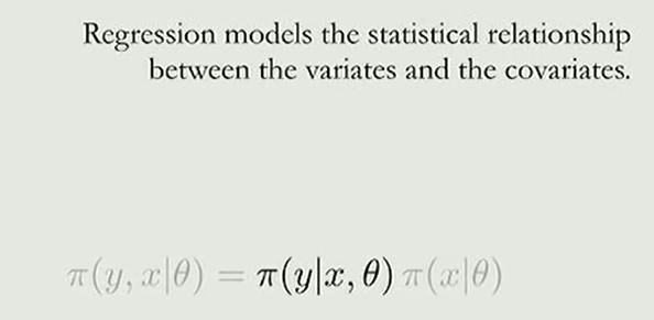
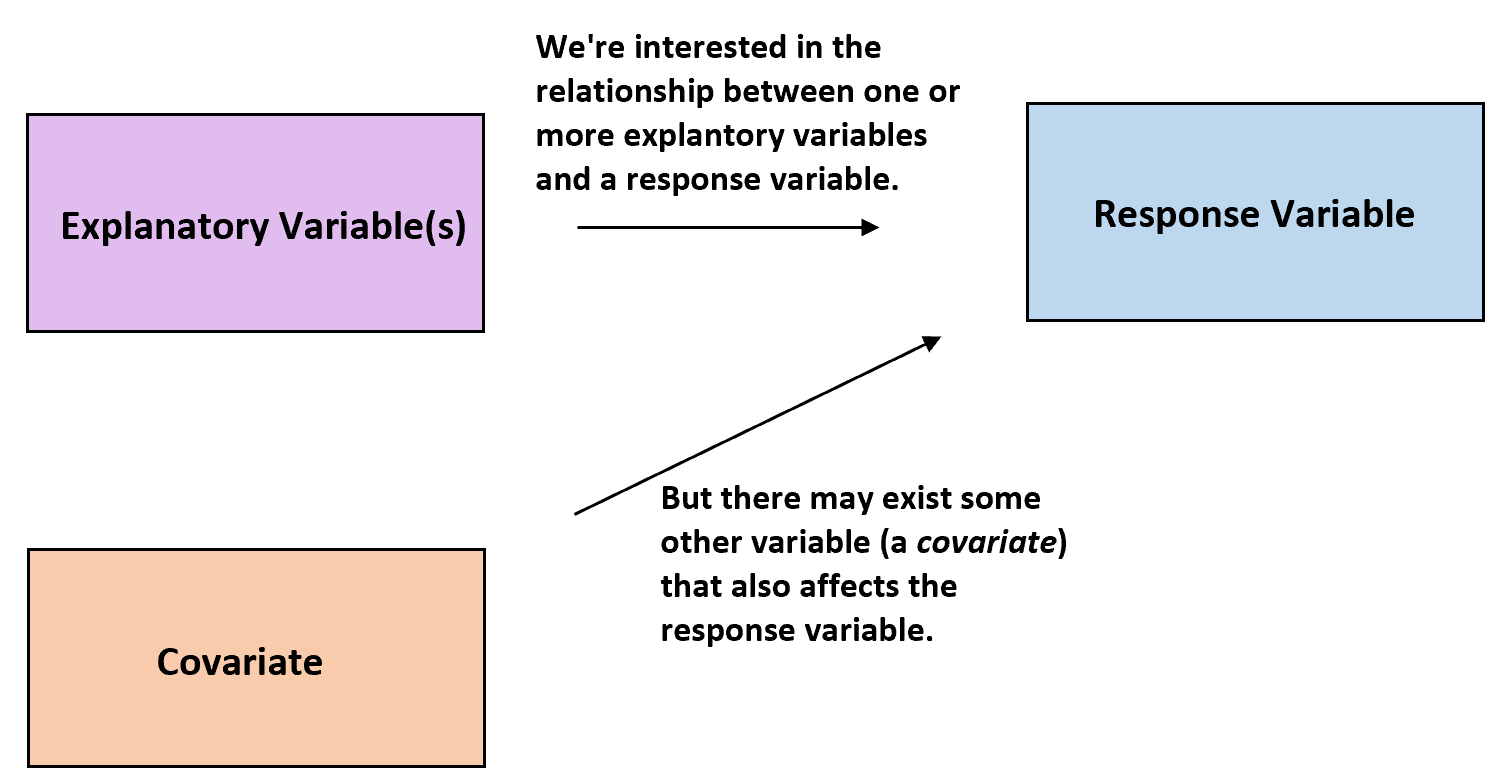
covariates

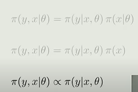
We typically assume that the covariates are independent of the model parameters.

Covariates(协变量): Variables that affect a response variable, but are not of interest in a study.

Covariates are often restricted to a single effective parameter through a deterministic mapping.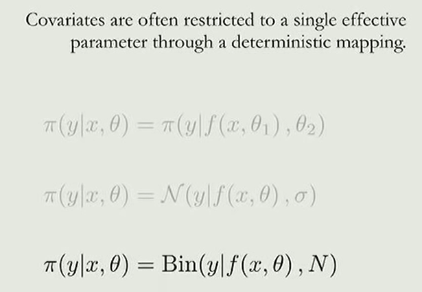

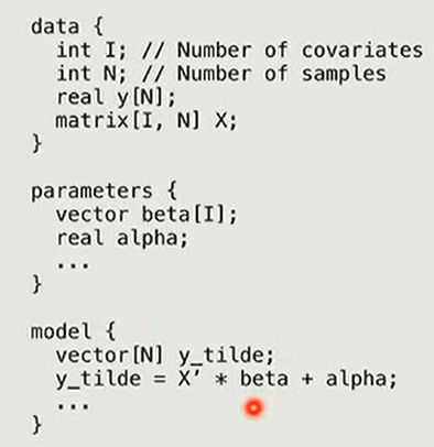
Multiple covariates are commonly encapsulated（压缩） in a design matrix.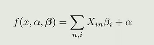

In collinearity some of the slopes are fully determined while the others are completely undetermined. 在共线情况下，一些坡度完全确定，而其他坡度则完全未确定。

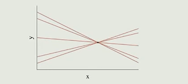
共线性那些事儿

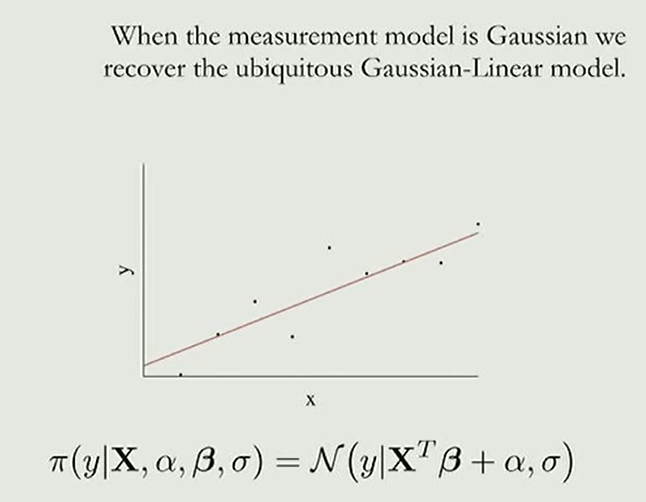
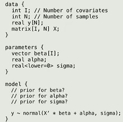
Consequently (weakly) informative priors are critical for building robust lincar models.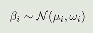

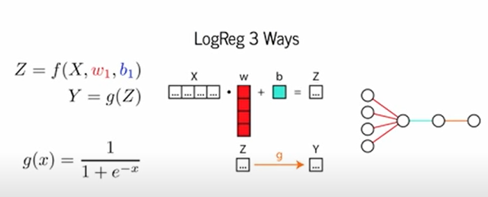
Bayesian Transforming

在一般的神经网络或一般的线性和逻辑回归中，我们所做的是学习一个参数，一个参数的估计，这个参数可以帮助我们最好地解释数据是什么样子。当我们谈论贝叶斯时，我们不把这个参数当作一个单独的待估计的东西，而是一个随机变量其他需要估计的参数，比如平均值和标准偏差，或者类似的东西，所以我们真正想要做的是，我们试图了解参数空间上的概率密度。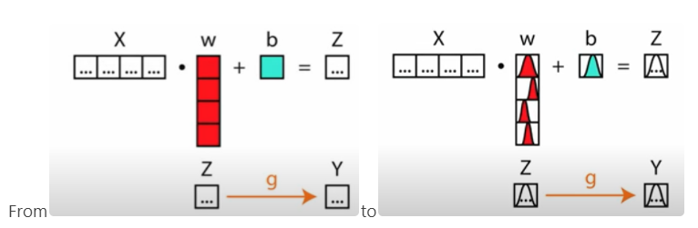

Hierarchical models

Confusing Statistical Term #4: Hierarchical Regression vs. Hierarchical Model

wikipedia/Multilevel_model
可视化 An Introduction to Hierarchical Modeling

What

等级线性模型（Hierarchical Linear Model、简称 HLM，也被称为mixed-effect model，random-effect models，nested data models或者multilevel linear models）

• 在计量经济学文献中也常常被称为Random-coefficient regression models
• 在某些统计学文献种也被称为Covariance components models

作用：An approach for modeling nested data.
等级线性模型特别适用于参与者的数据被组织在一个以上层次的研究设计（例如嵌套数据）。

Nested Data

Instances in which each observation is a member of a group, and you believe that group membership has an important effect on your outcome of interest.
每个观察的实例都是一个群体的成员，并且所属群体对结果具有重要影响。该模型的分析单位通常是在较低层次上的个人，他们被嵌套在较高层次上的背景或综合单位中。

作用：**这种数据结构导致了经典回归分析的独立性假设遭到违反。**

下文给出一个“教职员工薪资和部门的关系”的例子进行延展：

Estimating faculty salaries, where the faculty work in different departments. The group (department) that a faculty member belongs to could determine their salary in different ways. In this example, we’ll consider faculty who work in the Informatics, English, Sociology, Biology, and Statistics departments.

A Linear Approach

如果我们想用线性模型估计，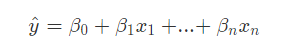
实际上就是在estimate the parameters (beta values)

These are known as the fixed effects because they are constant (fixed) for each individual.

本案例，我们可以用简单表示为：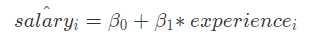

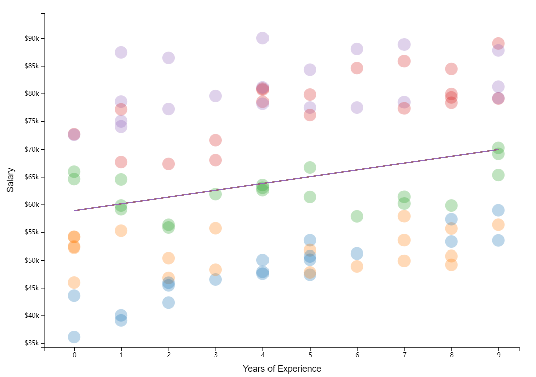
很明显的是，部门之间具有显著差异

这可能是因为“部门起薪”不同，可以通过改变截距（intercept）来解决：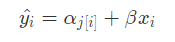

In the above equation, the vector of fixed effects (constant slopes) is represented by β , while the set of random intercepts is captured by α.

fixed effects (constant slopes)——> mixed model(random intercepts)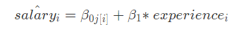

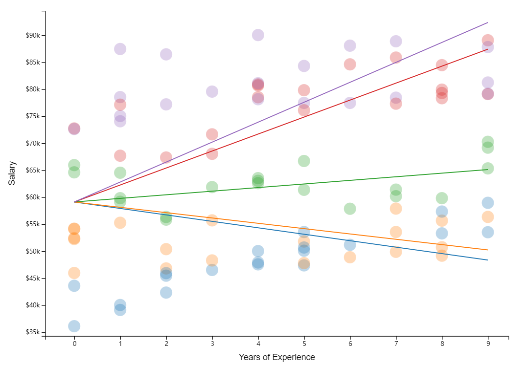
Random Slopes

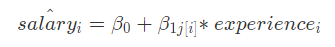
另外，我们也可以假设部门“涨薪水平”不一样，这可以通过改变斜率（slope）来模拟：
The intercept (β0) is constant(fixed) for all individuals, but the slope (βj) varies
——>

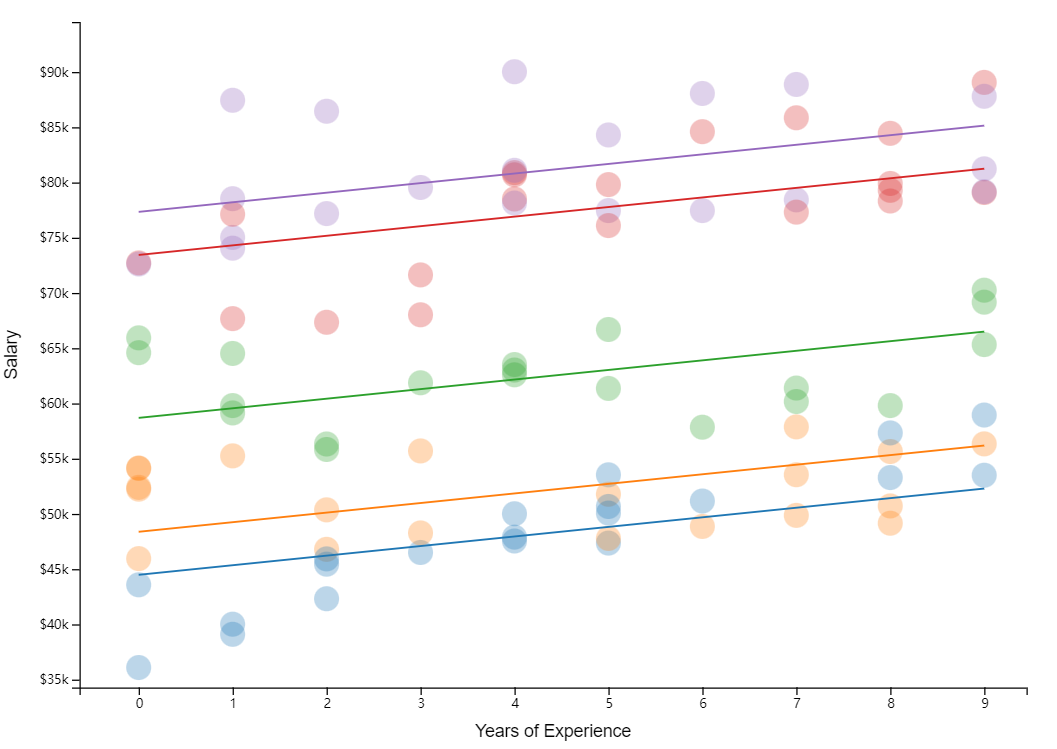
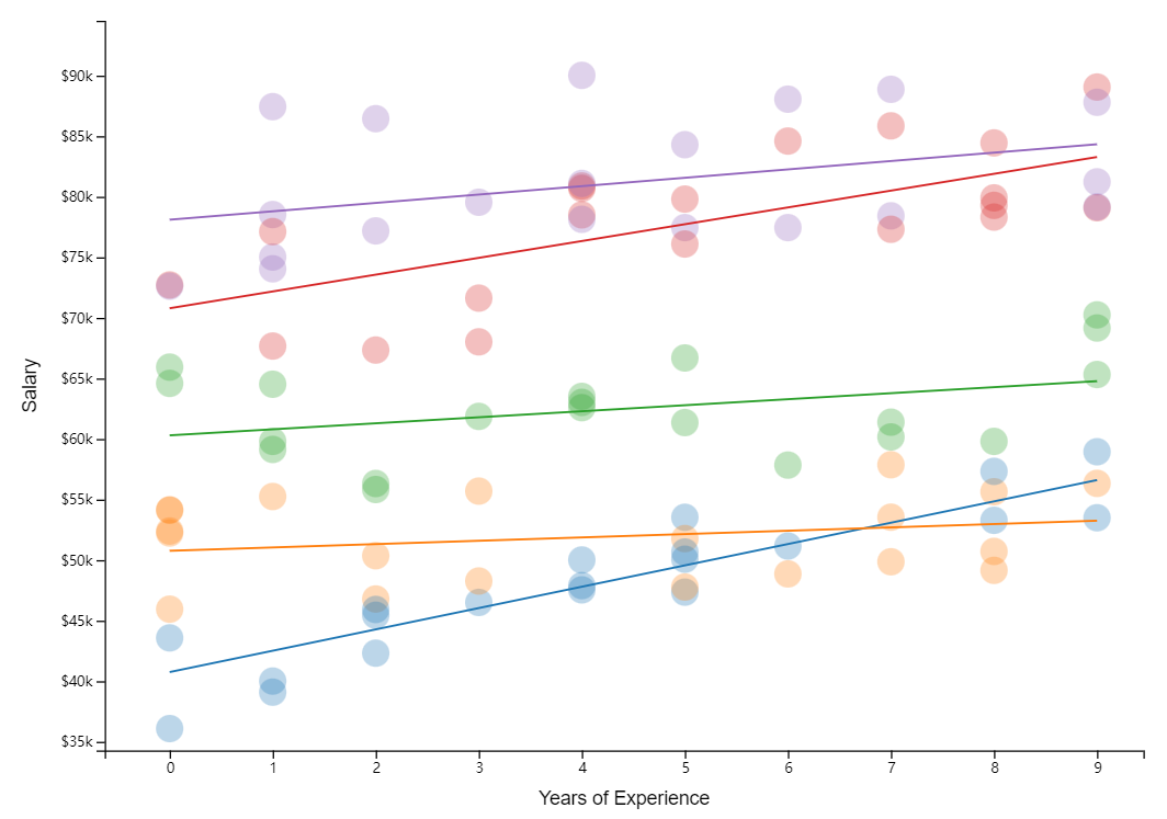
Random Slopes + Intercepts

把以上两个思想结合起来，问题就是变成：

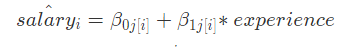
Faculty salaries start at different levels and increase at different rates depending on their department.

Thus, the starting salary for faculty member depends on their department (iαj[i]) ,
their annual raise also varies by department (βj[i].) :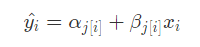
——>

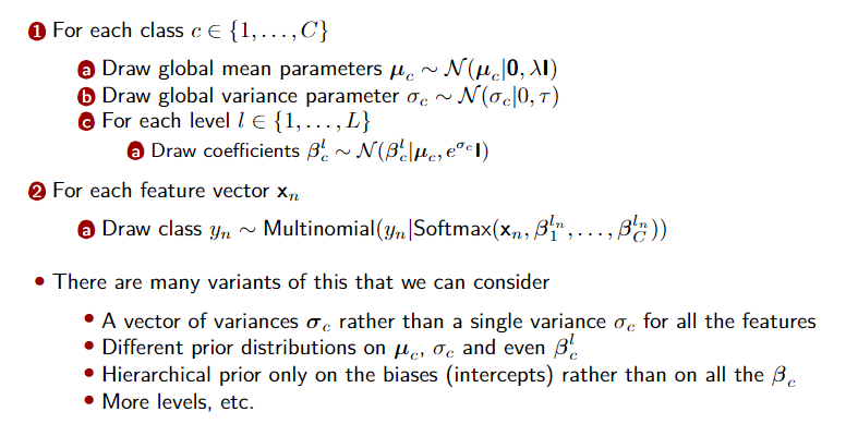
Hierarchical logistic regression model

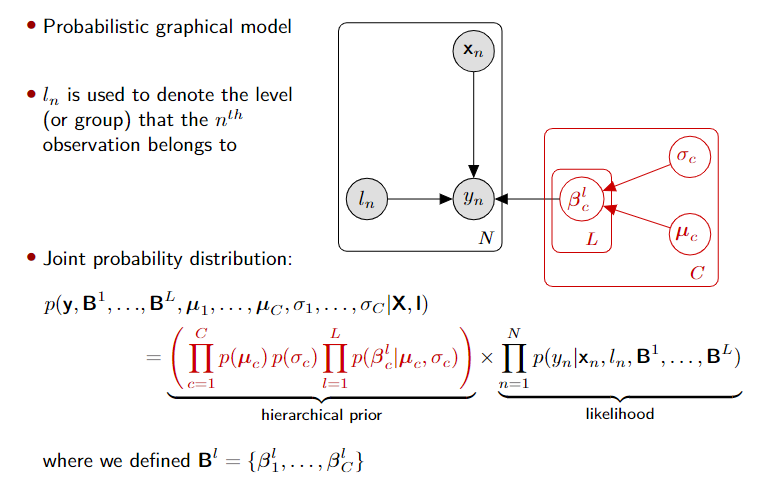
Generatice process

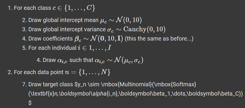
# define Stan model
model_definition = """
// TODO
data{
  int<lower=1> C; // number of classes
  int<lower=0> N; // number of data items/observations
  int<lower=1> D; // number of predictors
  int<lower=1> I; // numebr of individuals
  int<lower=1> ind[N]; // info about individual
  matrix[N,D] X;  // predictor matrix
  int<lower=1,upper=C> y[N]; // classes vector
}
parameters{
  vector[C] mu_prior;
  vector<lower=0>[C] sigma_prior;
  matrix[C,I] alpha;  // intercepts (biases) for each individual 
  matrix[C,D] beta;  // coefficients for predictors
}
model{
  for (c in 1:C){
    mu_prior[c] ~ normal(0,10); // hyper-prior on the intercepts mean
    sigma_prior[c] ~ cauchy(0,10); // hyper-prior on the intercepts variance
    beta[c] ~ normal(0,10);   // prior on the coefficients
    for (i in 1:I)
      alpha[c,i] ~ normal(mu_prior[c],sigma_prior[c]);
  }
  for (n in 1:N){
    y[n] ~ categorical(softmax(alpha[:,ind[n]]+beta*X[n]'])); // likelihood
  }
}
"""