Classification and Representation
Classification
Where y is a discrete value
- Develop the logistic regression algorithm to determine what class a new input should fall into
Classification problems
- Email -> spam/not spam?
- Online transactions -> fraudulent?
- Tumor -> Malignant/benign
Variable in these problems is Y
- Y is either 0 or 1
- 0 = negative class (absence of something)
- 1 = positive class (presence of something)

二分类问题
How do we develop a classification algorithm?
- Tumour size vs malignancy (0 or 1)
- We could use linear regression
- Then threshold the classifier output (i.e. anything over some value is Yes, else No)
- In our example below linear regression with thresholding seems to work

为什么线性回归不适用?/ 为什么要用逻辑回归?
- If we had a single Yes with _a very small tumour, _this would lead to classifying all the existing yeses as nos
- We know Y is 0 or 1. Hypothesis can give values large than 1 or less than 0
- logistic regression generates a value where is always either 0 or 1
多分类问题之后讨论
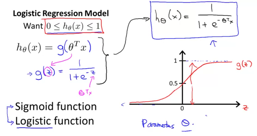
Hypothesis Representation
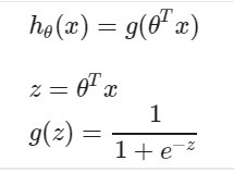
- What function is used to represent our hypothesis in classification
- We want our classifier to output values between 0 and 1
- Sigmoid function/ logistic function
Interpreting hypothesis output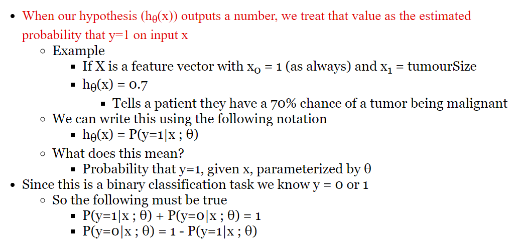
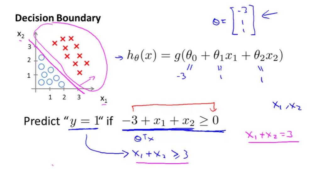
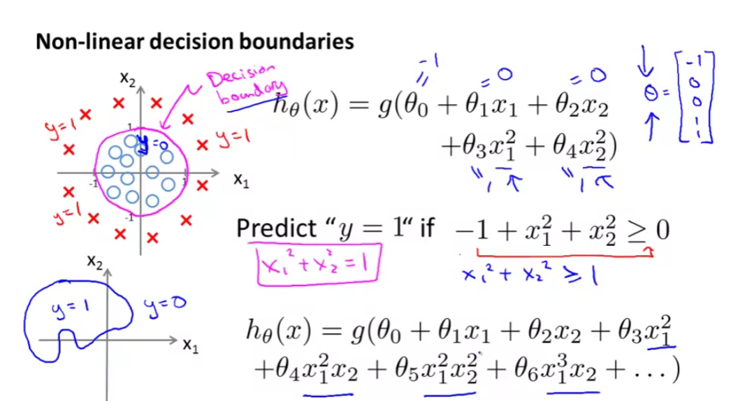
Decision Boundary
The decision boundary is the line that separates the area where y = 0 and where y = 1. It is created by our hypothesis function.
- Gives a better sense of what the hypothesis function is computing
Better understand of what the hypothesis function looks like
- One way of using the sigmoid function is;
- When the probability of y being 1 is greater than 0.5 then we can predict y = 1
- Else we predict y = 0
- When is it exactly that hθ(x) is greater than 0.5?
- Look at sigmoid function
- g(z) is greater than or equal to 0.5 when z is greater than or equal to 0
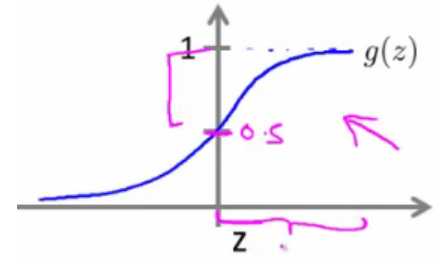
- So if z is positive, g(z) is greater than 0.5
- z = (θT x)
- So when
- θT x >= 0
- Then hθ >= 0.5
- Look at sigmoid function
- One way of using the sigmoid function is;
So what we’ve shown is that the hypothesis predicts y = 1 when θTx >= 0
- The corollary of that when θT x <= 0 then the hypothesis predicts y = 0
- Let’s use this to better understand how the hypothesis makes its predictions
Logistic Regression Model
复习:输入变量与输出变量均为连续变量的预测问题是回归问题,输出变量为有限个离散变量的预测问题成为分类问题。
使用线性的函数来拟合规律后取阈值,拟合的函数太直,离群值对结果的影响过大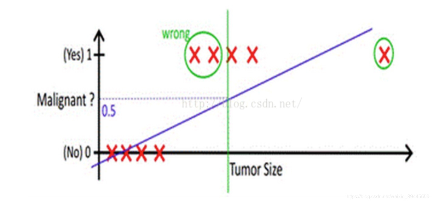
解决方法:
- 找到一个办法解决掉回归的函数严重受离群值影响的办法.
- 选定一个阈值.
Logistics regression是用来做分类任务的,为什么叫回归呢?
逻辑回归就是用回归的办法来做分类
Cost function for logistic regression
- Fit θ parameters
- Define the optimization object for the cost function we use the fit the parameters
- Training set of m training examples
- Each example has is n+1 length column vector
- Training set of m training examples
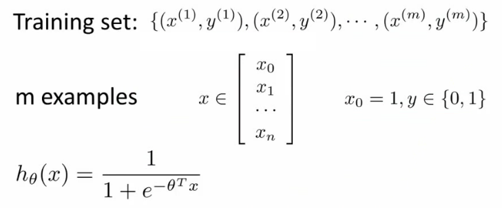
This is the situation
- Set of m training examples
- Each example is a feature vector which is n+1 dimensional
- x0 = 1
- y ∈ {0,1}
- Hypothesis is based on parameters (θ)
- Given the training set how to we chose/fit θ?
Linear regression uses the following function to determine θ
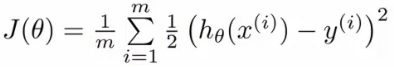
- Instead of writing the squared error term, we can write
- If we define “cost()” as;
- cost(hθ(xi), y) = 1/2(hθ(xi) - yi)2
- Which evaluates to the cost for an individual example using the same measure as used in linear regression
- We can redefine J(θ) as
- Which, appropriately, is the sum of all the individual costs over the training data (i.e. the same as linear regression)
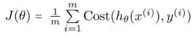
- If we define “cost()” as;
**
- What does this actually mean?
- This is the cost you want the learning algorithm to pay if the outcome is hθ(x) and the actual outcome is y
- If we use this function for logistic regression this is a non-convex function for parameter optimization
- Could work….
- What do we mean by non convex?
- We have some function - J(θ) - for determining the parameters
- Our hypothesis function has a non-linearity (sigmoid function of hθ(x) )
- This is a complicated non-linear function
- If you take hθ(x) and plug it into the Cost() function, and them plug the Cost() function into J(θ) and plot J(θ) we find many local optimum -> non convex function
- Why is this a problem
- We cannot use the same cost function that we use for linear regression because the Logistic Function will cause the output to be wavy, causing many local optima. In other words, it will not be a convex function.
- We would like a convex function so if you run gradient descent you converge to a global minimum
A convex logistic regression cost function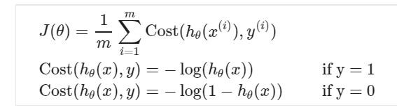
Cost function when y = 1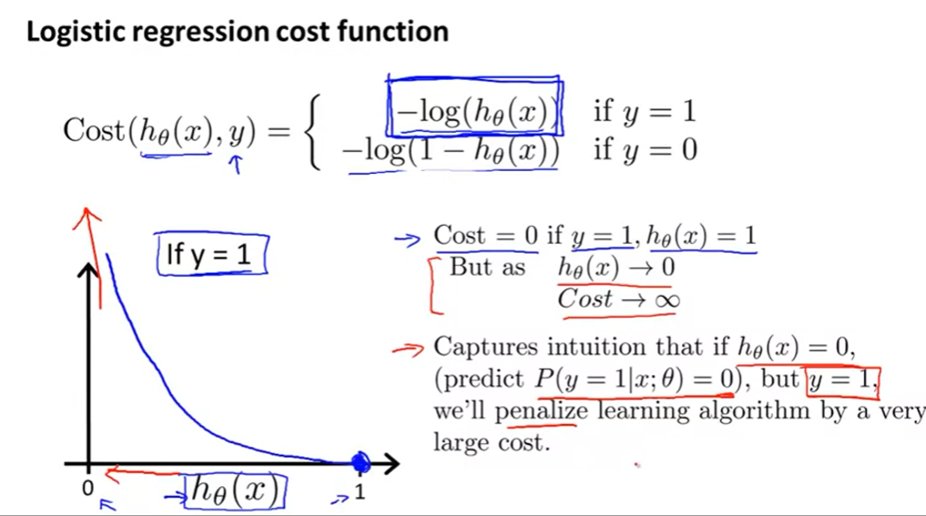
Cost function when y = 0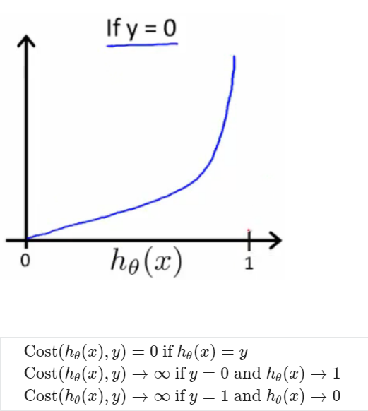
Simplified Cost Function and Gradient Descent
我们已经知道逻辑回归的损失函数如下: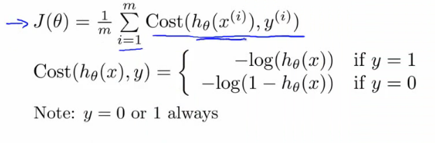
因为y要么是0,要么是1,我们可以将cost function合并简化成一个: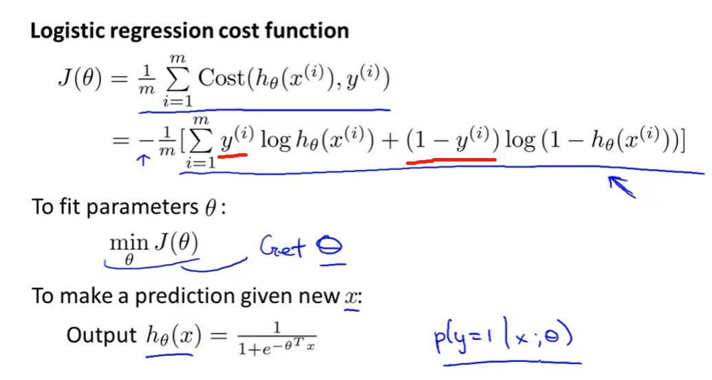
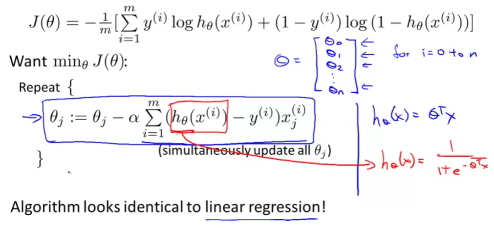
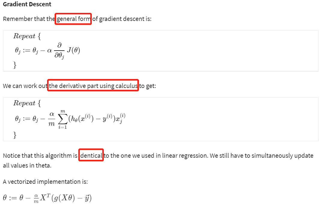
Gradient Descent
Advanced Optimization
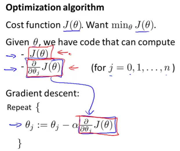
- Alternatively, instead of gradient descent to minimize the cost function we could use
- Conjugate gradient
- BFGS (Broyden-Fletcher-Goldfarb-Shanno)
- L-BFGS (Limited memory - BFGS)
- These are more optimized algorithms which take that same input and minimize the cost function
- These are _very _complicated algorithms
- Some properties
- Advantages
- No need to manually pick alpha (learning rate)
- Have a clever inner loop (line search algorithm) which tries a bunch of alpha values and picks a good one
- Often faster than gradient descent
- Do more than just pick a good learning rate
- Can be used successfully without understanding their complexity
- No need to manually pick alpha (learning rate)
- Disadvantages
- Could make debugging more difficult
- Should not be implemented themselves
- Different libraries may use different implementations - may hit performance
- Advantages

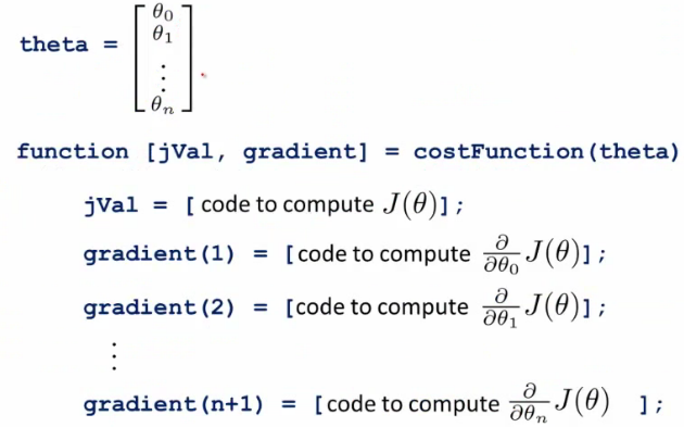
function [jval, gradent] = costFunction(THETA)
- Input for the cost function is THETA, which is a vector of the θ parameters
- Two return values from costFunction are
- jval
- How we compute the cost function θ (the underived cost function)
- In this case = (θ1 - 5)2 + (θ2 - 5)2
- How we compute the cost function θ (the underived cost function)
- gradient
- 2 by 1 vector
- 2 elements are the two partial derivative terms
- i.e. this is an n-dimensional vector
- Each indexed value gives the partial derivatives for the partial derivative of J(θ) with respect to θi
- Where i is the index position in the gradient vector
- jval
With the cost function implemented, we can call the advanced algorithm using
options= optimset('GradObj', 'on', 'MaxIter', '100'); # define the options data structureinitialTheta= zeros(2,1); # set the initial dimensions for theta # initialize the theta values[optTheta, funtionVal, exitFlag]= fminunc(@costFunction, initialTheta, options); # run the algorithm
Here
- options is a data structure giving options for the algorithm
- fminunc
- function minimize the cost function (find minimum of unconstrained multivariable function)
- @costFunction is a pointer to the costFunction function to be used
- For the octave implementation
- initialTheta must be a matrix of at least two dimensions
- How do we apply this to logistic regression?
- Here we have a vector
- Here
- theta is a n+1 dimensional column vector
- Octave indexes from 1, not 0
- Write a cost function which captures the cost function for logistic regression
Multiclass Classification
- Getting logistic regression for multiclass classification using one vs. all
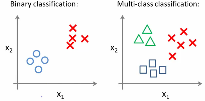
- Given a dataset with three classes, how do we get a learning algorithm to work?
- Use one vs. all classification make binary classification work for multiclass classification
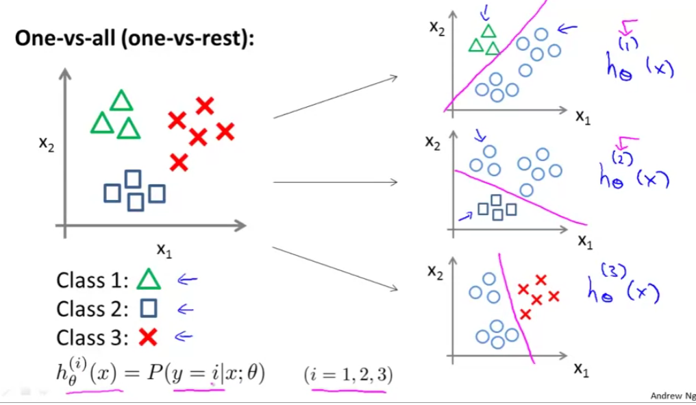
- One vs. all classification
- Split the training set into three separate binary classification problems
- i.e. create a new fake training set
- Triangle (1) vs crosses and squares (0) hθ1(x)
- P(y=1 | x1; θ)
- Crosses (1) vs triangle and square (0) hθ2(x)
- P(y=1 | x2; θ)
- Square (1) vs crosses and square (0) hθ3(x)
- P(y=1 | x3; θ)
- Triangle (1) vs crosses and squares (0) hθ1(x)
- i.e. create a new fake training set
- Split the training set into three separate binary classification problems
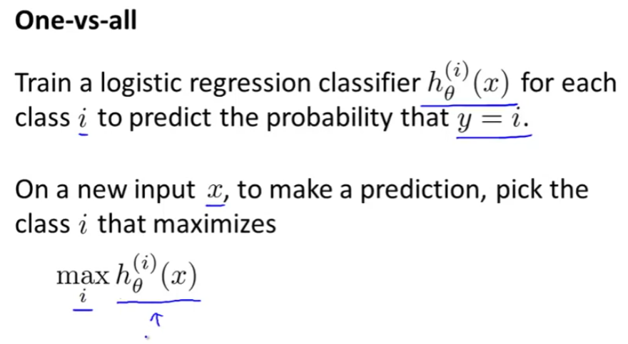
To summarize
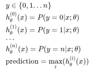
- Train a logistic regression classifier hθ(i)(x) for each class i to predict the probability that y = i
- On a new input, x to make a prediction, pick the class i that maximizes the probability that hθ(i)(x) = 1
Slides

若有收获,就点个赞吧
0 人点赞
