Learning Goals
- determine which features are the most important with mutual information
- invent new features in several real-world problem domains
- encode high-cardinality categoricals with a target encoding
- create segmentation features with k-means clustering
- decompose a dataset’s variation into features with principal component analysis
1 What Is Feature Engineering
Learn the steps and principles of creating better features
The Goal of Feature Engineering
The goal of feature engineering is simply to make your data better suited to the problem at hand.
You might perform feature engineering to:
- improve a model’s predictive
- reduce computational or data needs
- improve interpretability(可解释性) of the results
A Guiding Principle of Feature Engineering
- 有用的特征必须和模型目标有关
- 应用于特征的转换实质上会成为模型本身的一部分
Establishing baselines like this is good practice at the start of the feature engineering process.
A baseline score can help you decide whether your new features are worth keeping, or whether you should discard them and possibly try something else.
2 Mutual Information 互信息
Locate features with the most potential.
当拿到一个新数据集的时候常常感到压力山大,面对成百上千的特征手足无措。
第一步我们可以建立:feature utility metric, a function measuring associations between a feature and the target.
Mutual information is a lot like correlation in that it measures a relationship between two quantities. (变量间相互依赖性的量度)
The advantage of mutual information is that it can detect any kind of relationship, while correlation(相关性) only detects linear relationships.
特点:
- easy to use and interpret,
- computationally efficient,
- theoretically well-founded,
- resistant to overfitting, and,
- able to detect any kind of relationship
Mutual Information and What it Measures
Mutual information describes relationships in terms of uncertainty.
The mutual information (MI) between two quantities is a measure of the extent to which knowledge of one quantity reduces uncertainty about the other.(衡量随一个随机变量的了解程度加深,其他变量不确定性减少的程度)
延伸:(Information gain)表示得知特征X的信息而使得类Y的信息的不确定性减少的程度. —般地,熵H(Y)与条件熵H(Y|X)之差称为互信息(mutual information) 决策树学习中的信息增益等价于训练数据集中类与特征的互信息. 更多:李航-统计学习方法PPT-第四章贝叶斯分类器-P79
举例:如图展示房子外部品质与房子售价的关系,每个点代表一个房。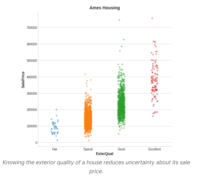
Technical note
- What we’re calling uncertainty is measured using a quantity from information theory known as “entropy(熵,即混乱、无序程度)”.
- The entropy of a variable means roughly: “how many yes-or-no questions you would need to describe an occurance of that variable, on average.”
- The more questions you have to ask, the more uncertain you must be about the variable.
- Mutual information is how many questions you expect the feature to answer about the target.
Interpreting Mutual Information Scores
MI最小值是0.0,当MI为0时,变量间相互独立,互不依赖;
理论上,MI无上限,但超过2是不常见,因为MI是个对数量。
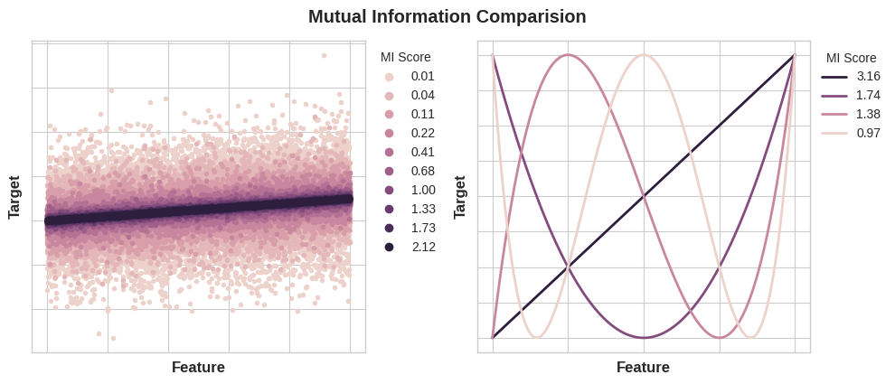
Left: Mutual information increases as the dependence between feature and target becomes tighter.
Right: Mutual information can capture any kind of association (not just linear, like correlation.)
Things to remember when applying mutual information:
- MI可以帮助您了解特征作为目标预测因子的相对潜力
- MI无法探测特征之间的交互,它是一个单变量度量
- 特征的作用取决于你使用的模型,只有当特征和目标的关系可以被模型学习时才有用,因为很高的MI并不意味模型能起什么作用,你需要先transform特征去暴露他们之间的联系
Scikit-learn has two mutual information metrics in its feature_selection module:
- one for real-valued targets (
mutual_info_regression) - one for categorical targets (
mutual_info_classif). ```python from sklearn.feature_selection import mutual_info_regression
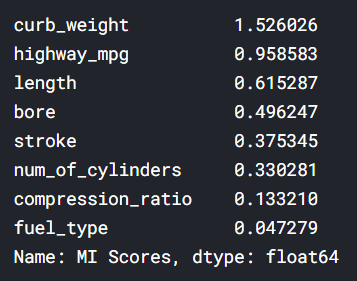
def make_mi_scores(X, y, discrete_features): mi_scores = mutual_info_regression(X, y, discrete_features=discrete_features) mi_scores = pd.Series(mi_scores, name=”MI Scores”, index=X.columns) mi_scores = mi_scores.sort_values(ascending=False) return mi_scores
mi_scores = make_mi_scores(X, y, discrete_features) mi_scores[::3] # show a few features with their MI scores
A bar plot to make comparisions```pythondef plot_mi_scores(scores):scores = scores.sort_values(ascending=True)width = np.arange(len(scores))ticks = list(scores.index)plt.barh(width, scores)plt.yticks(width, ticks)plt.title("Mutual Information Scores")plt.figure(dpi=100, figsize=(8, 5))plot_mi_scores(mi_scores)
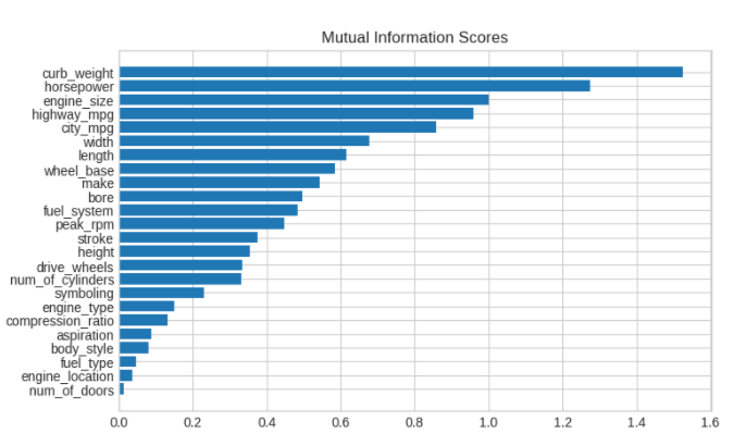
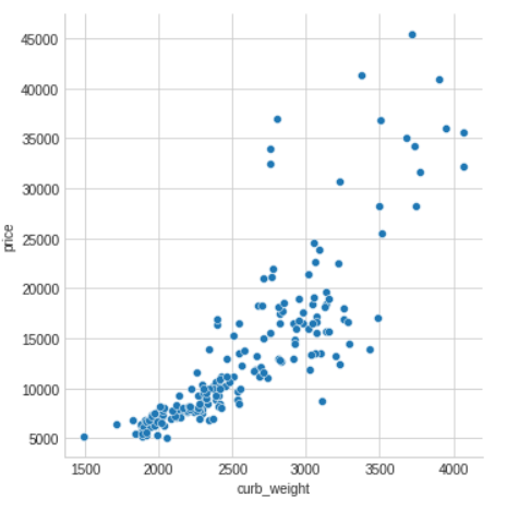
As we might expect, the high-scoring curb_weight feature exhibits a strong relationship with price, the target.
curb weight(汽车的整备质量)是指汽车按出厂技术条件装备完整(如备胎、工具等安装齐备),各种油水添满后的重量。
sns.relplot(x="curb_weight", y="price", data=df);
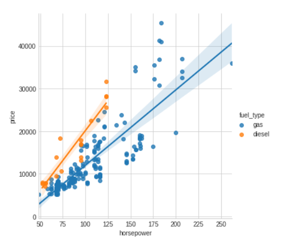
The fuel_type feature has a fairly low MI score, but as we can see from the figure, it clearly separates two price populations with different trends within the horsepower feature. This indicates that fuel_type contributes an interaction effect and might not be unimportant after all.
Before deciding a feature is unimportant from its MI score, it’s good to investigate any possible interaction effects — domain knowledge can offer a lot of guidance here.
sns.lmplot(x="horsepower", y="price", hue="fuel_type", data=df);
Example - House Prices
查看几个features与售价的关系
features = ["YearBuilt", "MoSold", "ScreenPorch"]
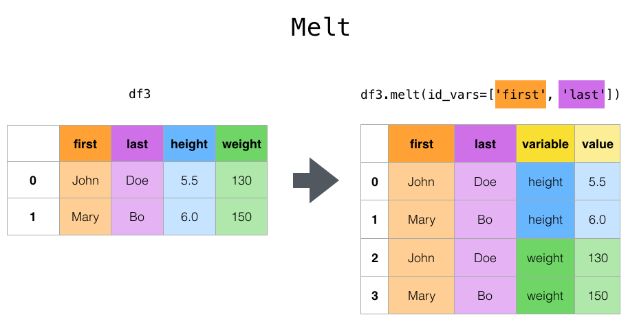
sns.relplot(
x="value", y="SalePrice", col="variable", data=df.melt(id_vars="SalePrice", value_vars=features), facet_kws=dict(sharex=False),
);
# replot出的图默认为散点图,
# col: 列上的子图(有多少种就显示多少个)
# df.melt() 是 df.pivot() 逆转操作函数
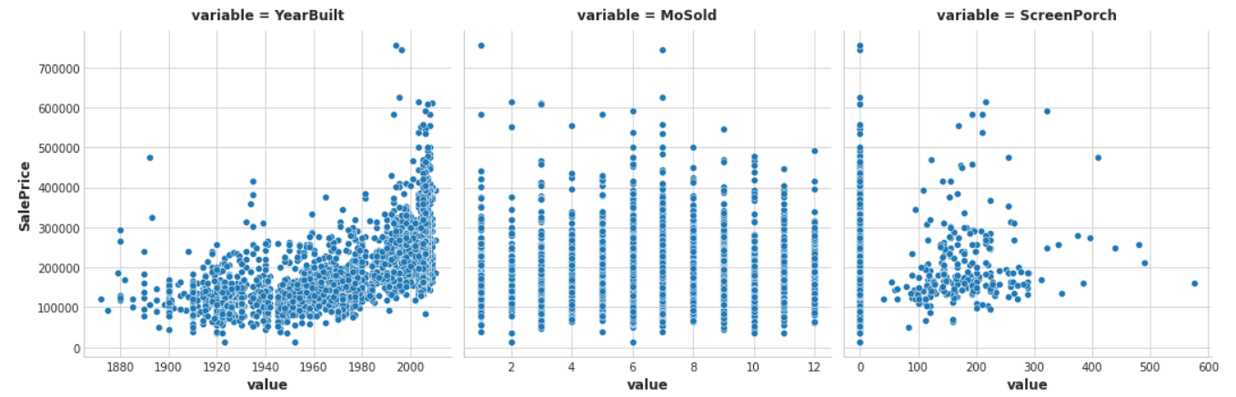
根据上图,YearBuilt的MI scores应该最高,因为Year倾向于将SalePrice约束在一个较集中的范围。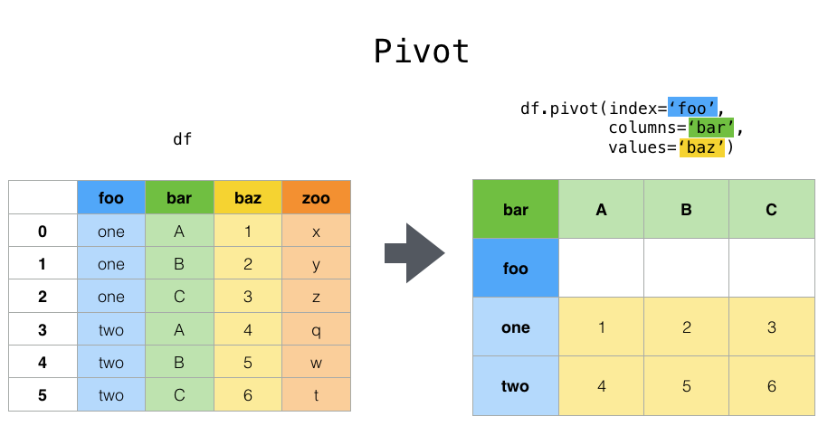
print(mi_scores.head(20))
print(mi_scores.tail(20))  # uncomment to see bottom 20

#plt.figure(dpi=100, figsize=(8, 12))
#plot_mi_scores(mi_scores) # 总体MI分数的排行
plt.figure(dpi=100, figsize=(8, 5))
plot_mi_scores(mi_scores.head(20))
plot_mi_scores(mi_scores.tail(20))  # uncomment to see bottom 20
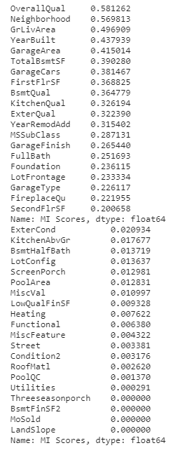

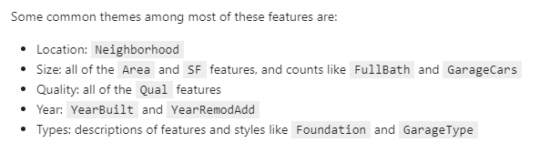
这些都是你在房地产列表中常见的特性(比如Zillow),我们的互信息度量对它们的评分很高。
另一方面,排名最低的功能似乎大多代表的东西是罕见的或特殊的某种方式,因此与一般购房者不太相关。
In this step you’ll investigate possible interaction effects for the BldgType feature. This feature describes the broad structure of the dwelling in five categories:
Bldg Type (Nominal): Type of dwelling
- 1Fam Single-family Detached(独栋)
- 2FmCon Two-family Conversion(改造屋); originally built as one-family dwelling
- Duplx Duplex(复式)
- TwnhsE Townhouse End Unit(联派单元房)
- TwnhsI Townhouse Inside Unit
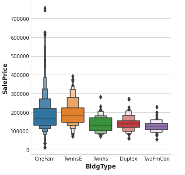
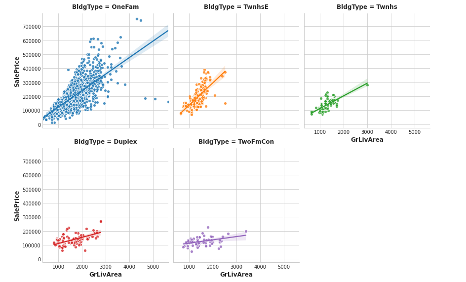
The BldgType feature didn’t get a very high MI score.
A plot confirms that the categories in BldgType don’t do a good job of distinguishing values in SalePrice (the distributions look fairly similar, in other words):
#catplot(): 用分类型数据(categorical data)绘图
sns.catplot(x="BldgType", y="SalePrice", data=df, kind="boxen");
feature1 = "GrLivArea"
sns.lmplot(
x=feature1, y="SalePrice", hue="BldgType", col="BldgType",
data=df, scatter_kws={"edgecolor": 'w'}, col_wrap=3, height=4,
);
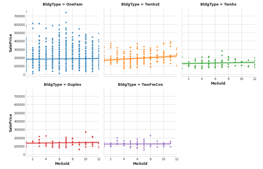
feature2 = "MoSold"
sns.lmplot(
x=feature2, y="SalePrice", hue="BldgType", col="BldgType",
data=df, scatter_kws={"edgecolor": 'w'}, col_wrap=3, height=4,
);
3 Creating Features
Transform features with Pandas to suit your model.
Tips on Discovering New Features
- Understand the features. Refer to your dataset’s data documentation, if available.
- Research the problem domain to acquire domain knowledge. If your problem is predicting house prices, do some research on real-estate for instance. Wikipedia can be a good starting point, but books and journal articles will often have the best information.
- Study previous work. Solution write-ups from past Kaggle competitions are a great resource.
- Use data visualization. Visualization can reveal pathologies in the distribution of a feature or complicated relationships that could be simplified. Be sure to visualize your dataset as you work through the feature engineering process.
import numpy as np
import pandas as pd
from sklearn.model_selection import cross_val_score
from xgboost import XGBRegressor

def score_dataset(X, y, model=XGBRegressor()):
    # Label encoding for categoricals
    for colname in X.select_dtypes(["category", "object"]):
        X[colname], _ = X[colname].factorize()
    # Metric for Housing competition is RMSLE (Root Mean Squared Log Error)
    score = cross_val_score(
        model, X, y, cv=5, scoring="neg_mean_squared_log_error",
    )
    score = -1 * score.mean()
    score = np.sqrt(score)
    return score


# Prepare data
df = pd.read_csv("../input/fe-course-data/ames.csv")
X = df.copy()
y = X.pop("SalePrice")
Mathematical Transforms
LivLotRatio: the ratio ofGrLivAreatoLotAreaSpaciousness: the sum ofFirstFlrSFandSecondFlrSFdivided byTotRmsAbvGrdTotalOutsideSF: the sum ofWoodDeckSF, OpenPorchSF, EnclosedPorch, Threeseasonporch, and ScreenPorch```python X_1 = pd.DataFrame() # dataframe to hold new features
X_1[“LivLotRatio”] = df.GrLivArea / df.LotArea X_1[“Spaciousness”] = (df[“FirstFlrSF”] + df[“SecondFlrSF”])/df[“TotRmsAbvGrd”] X_1[“TotalOutsideSF”] = df[“WoodDeckSF”]+df[“OpenPorchSF”]+df[“EnclosedPorch”]+df[“Threeseasonporch”]+df[“ScreenPorch”]
<a name="bPtUV"></a>
#### Interaction with a Categorical
```python
# One-hot encode BldgType. Use `prefix="Bldg"` in `get_dummies`
X_2 = pd.get_dummies(df.BldgType,prefix="Bldg")
# Multiply
X_2 = X_2.mul(df.GrLivArea,axis=0)
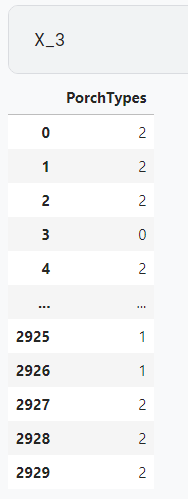
Counts
counts how many of the following are greater than 0.0:
X_3 = pd.DataFrame()

X_3["PorchTypes"] = df[[
    WoodDeckSF,
    OpenPorchSF,
    EnclosedPorch,
    Threeseasonporch,
    ScreenPorch
]].gt(0.0).sum(axis=1)
Building-Up and Breaking-Down Features
Break Down a Categorical Feature
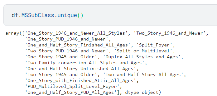
X_4 = pd.DataFrame()
X_4["MSClass"] = df.MSSubClass.str.split("_", n=1, expand=True)[0]

Group Transforms
Create a feature MedNhbdArea that describes the median of GrLivArea grouped on Neighborhood.
groupby函数详解
pandas分组与聚会
X_5 = pd.DataFrame()
X_5["MedNhbdArea"] = df.groupby("Neighborhood")["GrLivArea"].transform("median")
特征集合并
X_new = X.join([X_1, X_2, X_3, X_4, X_5])
score_dataset(X_new, y)
Tips on Creating Features
- It’s good to keep in mind your model’s own strengths and weaknesses when creating features. Here are some guidelines:
- Linear models learn sums and differences naturally, but can’t learn anything more complex.
- Ratios seem to be difficult for most models to learn. Ratio combinations often lead to some easy performance gains.
- Linear models and neural nets generally do better with normalized features. Neural nets especially need features scaled to values not too far from 0. Tree-based models (like random forests and XGBoost) can sometimes benefit from normalization, but usually much less so.
- Tree models can learn to approximate almost any combination of features, but when a combination is especially important they can still benefit from having it explicitly created, especially when data is limited.
- Counts are especially helpful for tree models, since these models don’t have a natural way of aggregating information across many features at once.
4 Clustering With K-Means
Untangle(理清) complex spatial relationships with cluster labels.
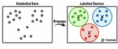
Clustering simply means the assigning of data points to groups based upon how similar the points are to each other. A clustering algorithm makes “birds of a feather flock together(物以类聚),” so to speak.
It’s important to remember that this Cluster feature is categorical.
分类方法有多种,主要差别在于measure “similarity” or “proximity” and in what kinds of features they work with.
- K-means clustering measures similarity using ordinary straight-line distance (Euclidean distance, in other words).
- It creates clusters by placing a number of points, called centroids, inside the feature-space.
- Each point in the dataset is assigned to the cluster of whichever centroid it’s closest to.
- The “k” in “k-means” is how many centroids (that is, clusters) it creates. You define the k yourself.
a simple two-step process
The algorithm starts by randomly initializing some predefined number (n_clusters) of centroids. It then iterates over these two operations:
- assign points to the nearest cluster centroid
- move each centroid to minimize the distance to its points
It iterates over these two steps until the centroids aren’t moving anymore, or until some maximum number of iterations has passed (max_iter).
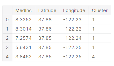
# Create cluster feature
kmeans = KMeans(n_clusters=6)
X["Cluster"] = kmeans.fit_predict(X)
X["Cluster"] = X["Cluster"].astype("category")

X.head()
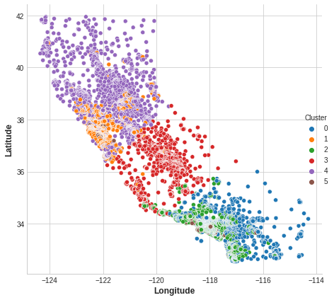
sns.relplot(
    x="Longitude", y="Latitude", hue="Cluster", data=X, height=6,
);
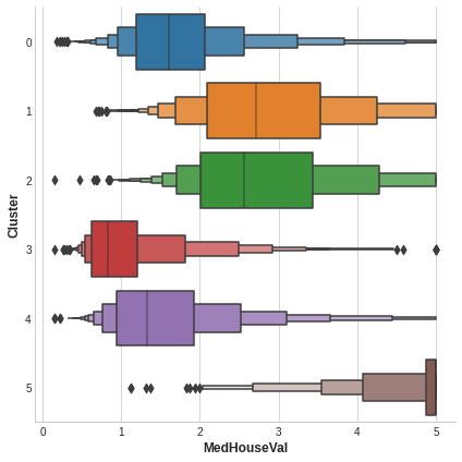
X["MedHouseVal"] = df["MedHouseVal"]
sns.catplot(x="MedHouseVal", y="Cluster", data=X, kind="boxen", height=6);
1 Scaling Features
k-means is sensitive to scale
This means we need to be thoughtful about how and whether we rescale our features since we might get very different results depending on our choices.
As a rule of thumb,
- 直接可比 (like a test result at different times), then you would not want to rescale.
- 不直接可比 (like height and weight) will usually benefit from rescaling.
Sometimes, the choice won’t be clear though. In that case, you should try to use common sense, remembering that features with larger values will be weighted more heavily.
判断是否需要rescaling
LatitudeandLongitudeof cities in CaliforniaLot AreaandLiving Areaof houses in Ames, IowaNumber of DoorsandHorsepowerof a 1989 model car不可rescale,因为会扭曲经纬度间的自然距离
- 都可以,因为单位一样,但是rescale之后在预测房价上LotArea对聚类就不会不成比例地影响
- 完全不可比,如果不rescale的话,房门数量(2/4)的权重与马力相比可能就会被忽视
Comparing different rescaling schemes through cross-validation can also be helpful. (You might like to check out the preprocessing module in scikit-learn for some of the rescaling methods it offers.)
2 Create a Feature of Cluster Labels
X = df.copy()
y = X.pop("SalePrice")


# YOUR CODE HERE: Define a list of the features to be used for the clustering
features = [
    "LotArea",
    ____,
    ____,
    ____,
    ____,
]

# Standardize
X_scaled = X.loc[:, features]
X_scaled = (X_scaled - X_scaled.mean(axis=0)) / X_scaled.std(axis=0)


# YOUR CODE HERE: Fit the KMeans model to X_scaled and create the cluster labels
kmeans = KMeans(n_clusters=____, n_init=____, random_state=0)
X["Cluster"] = kmeans.fit_predict(X_scaled)
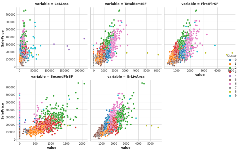
可视化聚类效果
Xy = X.copy()
Xy["Cluster"] = Xy.Cluster.astype("category")
Xy["SalePrice"] = y
sns.relplot(
    x="value", y="SalePrice", hue="Cluster", col="variable",
    height=4, aspect=1, facet_kws={'sharex': False}, col_wrap=3,
    data=Xy.melt(
        value_vars=features, id_vars=["SalePrice", "Cluster"],
    ),
);
score_dataset will score your XGBoost model with this new feature added to training data.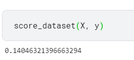
The k-means algorithm offers an alternative way of creating features.
Instead of labelling each feature with the nearest cluster centroid, it can measure the distance from a point to all the centroids and return those distances as features.
3 Cluster-Distance Features
Now add the cluster-distance features to your dataset. You can get these distance features by using the fit_transform method of kmeans instead of fit_predict.
kmeans = KMeans(n_clusters=10, n_init=10, random_state=0)


# YOUR CODE HERE: Create the cluster-distance features using `fit_transform`
X_cd = kmeans.fit_transform(X_scaled)


# Label features and join to dataset
X_cd = pd.DataFrame(X_cd, columns=[f"Centroid_{i}" for i in range(X_cd.shape[1])])
X = X.join(X_cd)
5 Principal Component Analysis(PCA)主成分分析
Discover new features by analyzing variation.
Introduction
The main idea of principal component analysis (PCA) is to reduce the dimensionality of a data set consisting of many variables correlated with each other, either heavily or lightly, while retaining the variation present in the dataset, up to the maximum extent.
PCA 是一种常见的数据分析方式,常用于高维数据的降维,可用于提取数据的主要特征分量。
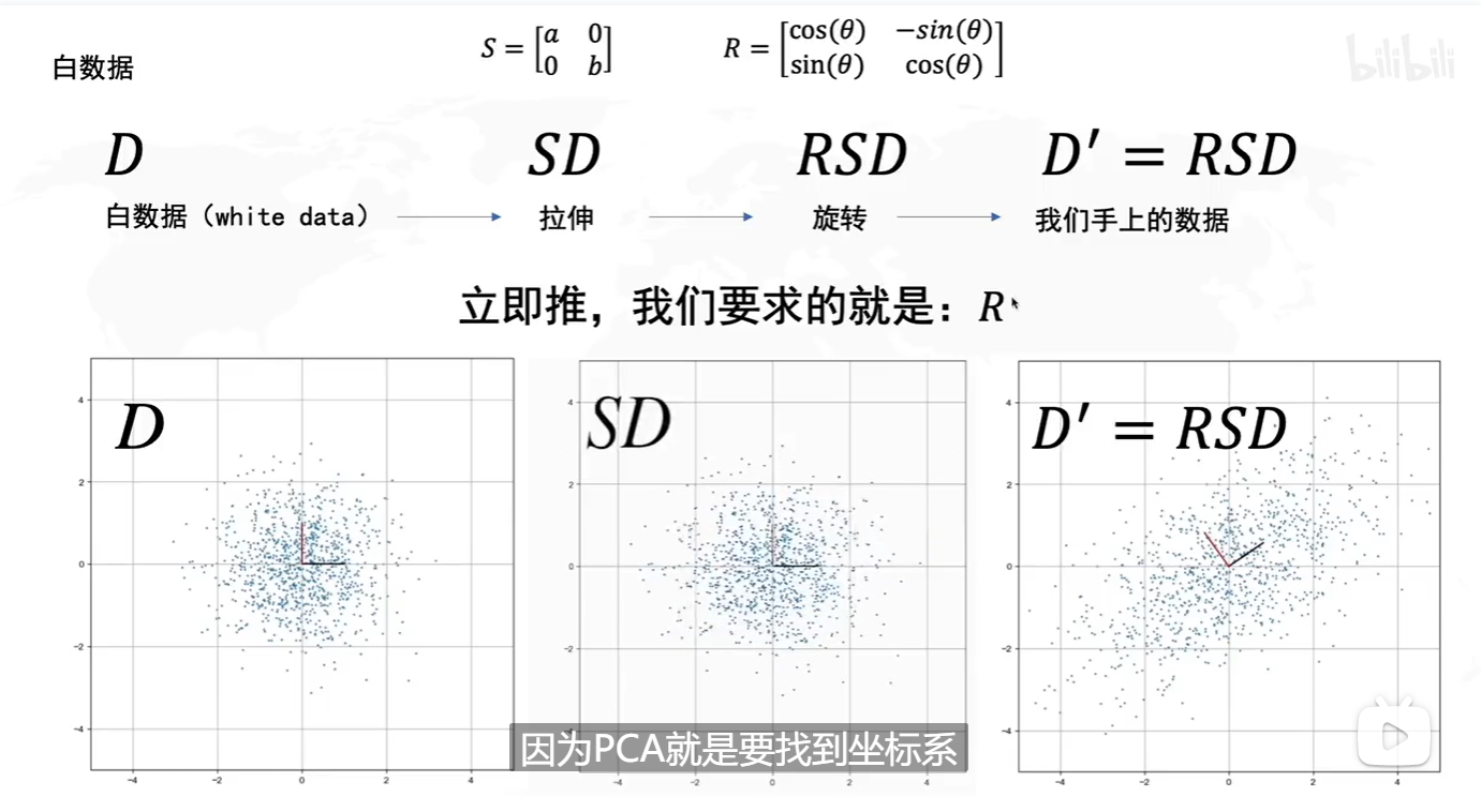
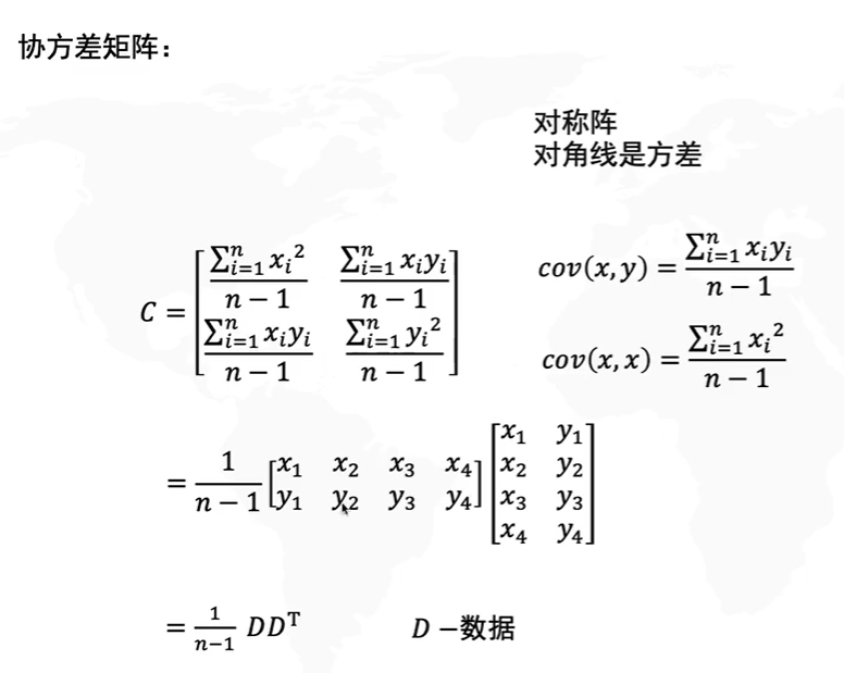
Technical note: PCA is typically applied to standardized data. With standardized data “variation” means “correlation”. With unstandardized data “variation” means “covariance(协方差)”. All data in this course will be standardized before applying PCA.
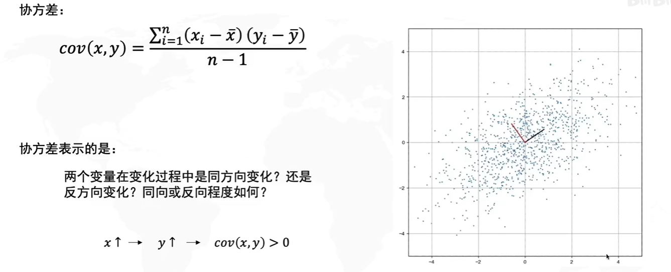
在一维空间中我们可以用方差来表示数据的分散程度。 而对于高维数据,我们用协方差进行约束,协方差可以表示两个变量的相关性。 为了让两个变量尽可能表示更多的原始信息,我们希望它们之间不存在线性相关性,因为相关性意味着两个变量不是完全独立,必然存在重复表示的信息。
Principal Component Analysis
The new features PCA constructs are actually just “linear combinations (weighted sums)” of the original features:
df["Size"] = 0.707 * X["Height"] + 0.707 * X["Diameter"]
df["Shape"] = 0.707 * X["Height"] - 0.707 * X["Diameter"]
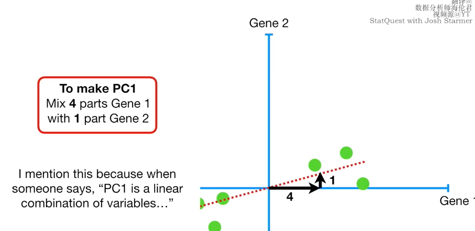
linear combination的解释
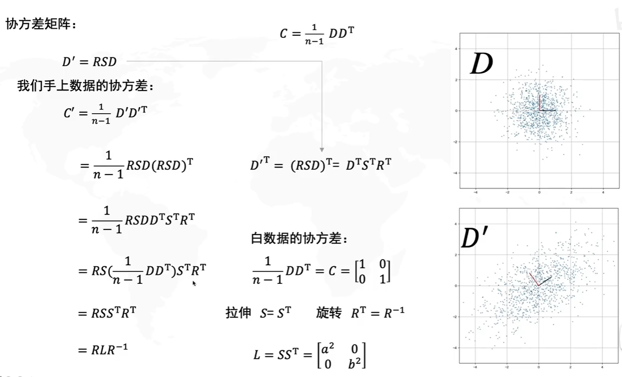
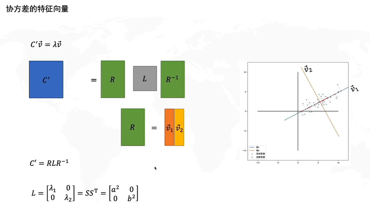
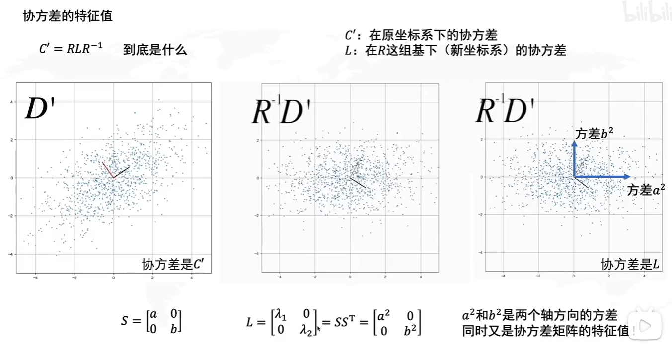
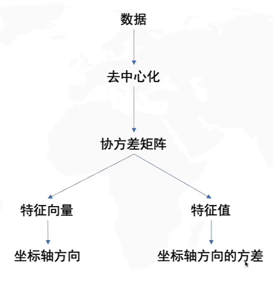
思考:我们如何得到这些包含最大差异性的主成分方向呢?
答案:通过计算数据矩阵的协方差矩阵,然后得到协方差矩阵的特征值、特征向量,选择特征值最大(即方差最大)的k个特征所对应的特征向量组成的矩阵。这样就可以将数据矩阵转换到新的空间当中,实现数据特征的降维。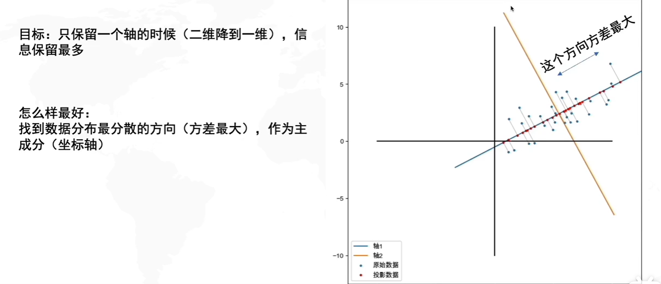
PCA for Feature Engineering
two ways
- 利用描述性技巧,计算MI分数看哪些变化对目标最有预测性
- 将自身模块作为features,
use-cases:
- Dimensionality reduction: When your features are highly redundant (multicollinear, specifically), PCA will partition out the redundancy into one or more near-zero variance components, which you can then drop since they will contain little or no information.
- Anomaly detection: Unusual variation, not apparent from the original features, will often show up in the low-variance components. These components could be highly informative in an anomaly or outlier detection task.
- Noise reduction: A collection of sensor readings will often share some common background noise. PCA can sometimes collect the (informative) signal into a smaller number of features while leaving the noise alone, thus boosting the signal-to-noise ratio.
- Decorrelation: Some ML algorithms struggle with highly-correlated features. PCA transforms correlated features into uncorrelated components, which could be easier for your algorithm to work with.
PCA求解步骤
两种方法:
- 基于特征值分解协方差矩阵实现PCA算法
- 基于SVD分解协方差矩阵实现PCA算法
PCA Best Practices
There are a few things to keep in mind when applying PCA:
- PCA only works with numeric features, like continuous quantities or counts.
- PCA is sensitive to scale. It’s good practice to standardize your data before applying PCA, unless you know you have good reason not to.
- Consider removing or constraining outliers, since they can an have an undue influence on the results.
缺点:离群点影响大
Example
def apply_pca(X, standardize=True):
    # Standardize
    if standardize:
        X = (X - X.mean(axis=0)) / X.std(axis=0)
    # Create principal components
    pca = PCA()
    X_pca = pca.fit_transform(X)
    # Convert to dataframe
    component_names = [f"PC{i+1}" for i in range(X_pca.shape[1])]
    X_pca = pd.DataFrame(X_pca, columns=component_names)
    # Create loadings
    loadings = pd.DataFrame(
        pca.components_.T,  # transpose the matrix of loadings
        columns=component_names,  # so the columns are the principal components
        index=X.columns,  # and the rows are the original features
    )
    return pca, X_pca, loadings


def plot_variance(pca, width=8, dpi=100):
    # Create figure
    fig, axs = plt.subplots(1, 2)
    n = pca.n_components_
    grid = np.arange(1, n + 1)
    # Explained variance
    evr = pca.explained_variance_ratio_
    axs[0].bar(grid, evr)
    axs[0].set(
        xlabel="Component", title="% Explained Variance", ylim=(0.0, 1.0)
    )
    # Cumulative Variance
    cv = np.cumsum(evr)
    axs[1].plot(np.r_[0, grid], np.r_[0, cv], "o-")
    axs[1].set(
        xlabel="Component", title="% Cumulative Variance", ylim=(0.0, 1.0)
    )
    # Set up figure
    fig.set(figwidth=8, dpi=100)
    return axs


def make_mi_scores(X, y):
    X = X.copy()
    for colname in X.select_dtypes(["object", "category"]):
        X[colname], _ = X[colname].factorize()
    # All discrete features should now have integer dtypes
    discrete_features = [pd.api.types.is_integer_dtype(t) for t in X.dtypes]
    mi_scores = mutual_info_regression(X, y, discrete_features=discrete_features, random_state=0)
    mi_scores = pd.Series(mi_scores, name="MI Scores", index=X.columns)
    mi_scores = mi_scores.sort_values(ascending=False)
    return mi_scores


def score_dataset(X, y, model=XGBRegressor()):
    # Label encoding for categoricals
    for colname in X.select_dtypes(["category", "object"]):
        X[colname], _ = X[colname].factorize()
    # Metric for Housing competition is RMSLE (Root Mean Squared Log Error)
    score = cross_val_score(
        model, X, y, cv=5, scoring="neg_mean_squared_log_error",
    )
    score = -1 * score.mean()
    score = np.sqrt(score)
    return score

df = pd.read_csv("../input/fe-course-data/ames.csv")
选择比较关联的特征
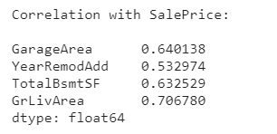
choose a few features that are highly correlated with our target, SalePrice.
features = [
    "GarageArea",
    "YearRemodAdd",
    "TotalBsmtSF",
    "GrLivArea",
]

print("Correlation with SalePrice:\n")
print(df[features].corrwith(df.SalePrice))
use PCA to untangle(整理) the correlational structure of these features and suggest relationships that might be usefully modeled with new features.
X = df.copy()
y = X.pop("SalePrice")
X = X.loc[:, features]
# `apply_pca`, defined above, reproduces the code from the tutorial
pca, X_pca, loadings = apply_pca(X)
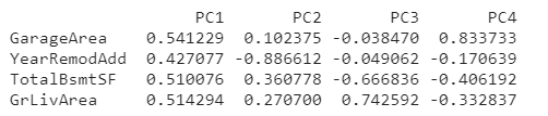
print(loadings)
1) Interpret Component Loadings
The first component, PC1, seems to be a kind of “size” component, similar to what we saw in the tutorial: all of the features have the same sign (positive), indicating that this component is describing a contrast between houses having large values and houses having small values for these features.
The interpretation of the third component PC3 is a little trickier. The features GarageArea and YearRemodAdd both have near-zero loadings, so let’s ignore those. This component is mostly about TotalBsmtSF and GrLivArea. It describes a contrast between houses with a lot of living area but small (or non-existant) basements, and the opposite: small houses with large basements.
Your goal in this question is to use the results of PCA to discover one or more new features that improve the performance of your model.
- to create features inspired by the loadings, like we did in the tutorial.
- or to use the components themselves as features (that is, add one or more columns of
X_pcatoX).
2) Create New Features
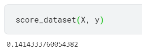
Add one or more new features to the dataset X.
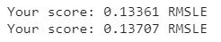
For a correct solution, get a validation score below 0.140 RMSLE.
# Solution 1: Inspired by loadings
X = df.copy()
y = X.pop("SalePrice")

X["Feature1"] = X.GrLivArea + X.TotalBsmtSF
X["Feature2"] = X.YearRemodAdd * X.TotalBsmtSF

score = score_dataset(X, y)
print(f"Your score: {score:.5f} RMSLE")


# Solution 2: Uses components
X = df.copy()
y = X.pop("SalePrice")

X = X.join(X_pca)
score = score_dataset(X, y)
print(f"Your score: {score:.5f} RMSLE")
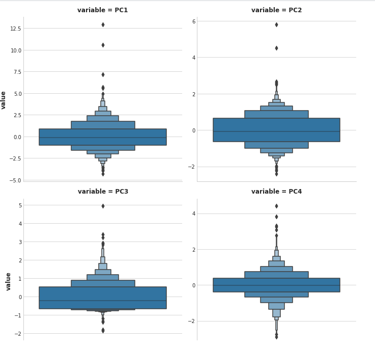
3) Outlier Detection
PCA in particular can show you anomalous(异常值) variation which might not be apparent from the original features: neither small houses nor houses with large basements are unusual, but it is unusual for small houses to have large basements.
sns.catplot(
    y="value",
    col="variable",
    data=X_pca.melt(),
    kind='boxen',
    sharey=False,
    col_wrap=2,
);
# You can change PC1 to PC2, PC3, or PC4
component = "PC1"

idx = X_pca[component].sort_values(ascending=False).index
df.loc[idx, ["SalePrice", "Neighborhood", "SaleCondition"] + features]
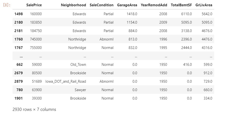
Notice that there are several dwellings listed as Partial sales in the Edwards neighborhood that stand out. A partial sale is what occurs when there are multiple owners of a property and one or more of them sell their “partial” ownership of the property.
These kinds of sales are often happen during the settlement of a family estate or the dissolution((官方组织的)解散;(法律合约的)解除) of a business and aren’t advertised publicly. If you were trying to predict the value of a house on the open market, you would probably be justified in removing sales like these from your dataset — they are truly outliers.
6 Target Encoding
- Boost any categorical feature with this powerful technique.
- a supervised feature engineering technique
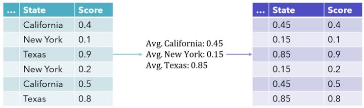
A target encoding is any kind of encoding that replaces a feature’s categories with some number derived from the target.
目标编码(Target encoding)是表示分类列的一种非常有效的方法,并且仅占用一个特征空间,也称为均值编码。该列中的每个值都被该类别的平均目标值替代。这可以更直接地表示分类变量和目标变量之间的关系。
目标编码(target encoding)
- 亦称均值编码(mean encoding)、似然编码(likelihood encoding)、效应编码(impact encoding)
- 是一种能够对高基数(high cardinality)自变量进行编码的方法 (Micci-Barreca 2001)
- 编码方式:有监督,如果运用得当则能够有效地提高预测模型的准确性 (Pargent, Bischl, and Thomas 2019) ;
- 关键:在编码的过程中引入正则化,避免过拟合问题。
高基数(High-Cardinality)的定义为在一个数据列中的数据基本上不重复,或者说重复率非常低。
缺点:
- 使模型更难学习均值编码变量和另一个变量之间的关系,仅基于列与目标的关系就在列中绘制相似性。
- 对 y 变量非常敏感,这会影响模型提取编码信息的能力
- 由于该类别的每个值都被相同的数值替换,因此模型可能会过拟合其见过的编码值(例如将 0.8 与完全不同的值相关联,而不是 0.79),这是把连续尺度上的值视为严重重复的类的结果。
Mean Encoding:
autos["make_encoded"] = autos.groupby("make")["price"].transform("mean")

autos[["make", "price", "make_encoded"]].head(10)
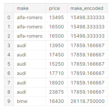
This kind of target encoding is sometimes called a mean encoding. Applied to a binary target, it’s also called bin counting. (Other names you might come across include: likelihood encoding, impact encoding, and leave-one-out encoding.)
Soomthing
label smoothing是一种在分类问题中,防止过拟合的方法。
An encoding like this presents a couple of problems.
- First are unknown categories.
Target encodings create a special risk of overfitting, which means they need to be trained on an independent “encoding” split. When you join the encoding to future splits, Pandas will fill in missing values for any categories not present in the encoding split. These missing values you would have to impute(估算) somehow.
- Second are rare categories.
When a category only occurs a few times in the dataset, any statistics calculated on its group are unlikely to be very accurate. In the Automobiles dataset, the mercurcy make only occurs once. The “mean” price we calculated is just the price of that one vehicle, which might not be very representative of any Mercuries we might see in the future. Target encoding rare categories can make overfitting more likely.
A solution to these problems is to add smoothing.
The idea is to blend the in-category average with the overall average. Rare categories get less weight on their category average, while missing categories just get the overall average.
In pseudocode(伪代码):
encoding = weight * in_category + (1 - weight) * overall
where weight is a value between 0 and 1 calculated from the category frequency.
An easy way to determine the value for weight is to compute an m-estimate:
weight = n / (n + m)
where n is the total number of times that category occurs in the data. The parameter m determines the “smoothing factor”. Larger values of m put more weight on the overall estimate.
In the Automobiles dataset there are three cars with the make chevrolet. If you chose m=2.0, then the chevrolet category would be encoded with 60% of the average Chevrolet price plus 40% of the overall average price.
chevrolet = 0.6 * 6000.00 + 0.4 * 13285.03
Use Cases for Target Encoding
Target encoding is great for:
- High-cardinality(高基数) features: A feature with a large number of categories can be troublesome to encode: a one-hot encoding would generate too many features and alternatives, like a label encoding, might not be appropriate for that feature. A target encoding derives numbers for the categories using the feature’s most important property: its relationship with the target.
- Domain-motivated features: From prior experience, you might suspect that a categorical feature should be important even if it scored poorly with a feature metric. A target encoding can help reveal a feature’s true informativeness.
Example - MovieLens1M
The MovieLens1M dataset contains one-million movie ratings by users of the MovieLens website, with features describing each user and movie. This hidden cell sets everything up:
Number of Unique Zipcodes: 3439
With over 3000 categories, the Zipcode feature makes a good candidate for target encoding, and the size of this dataset (over one-million rows) means we can spare some data to create the encoding.
We’ll start by creating a 25% split to train the target encoder.
X = df.copy()
y = X.pop('Rating')

X_encode = X.sample(frac=0.25)
y_encode = y[X_encode.index]
X_pretrain = X.drop(X_encode.index)
y_train = y[X_pretrain.index]
The category_encoders package in scikit-learn-contrib implements an m-estimate encoder, which we’ll use to encode our Zipcode feature.
from category_encoders import MEstimateEncoder

# Create the encoder instance. Choose m to control noise.
encoder = MEstimateEncoder(cols=["Zipcode"], m=5.0)

# Fit the encoder on the encoding split.
encoder.fit(X_encode, y_encode)

# Encode the Zipcode column to create the final training data
X_train = encoder.transform(X_pretrain)
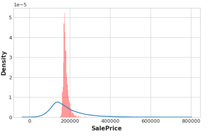
Let’s compare the encoded values to the target to see how informative our encoding might be.
plt.figure(dpi=90)
ax = sns.distplot(y, kde=False, norm_hist=True) #集合了matplotlib的hist()与sns.kdeplot()功能
ax = sns.kdeplot(X_train.Zipcode, color='r', ax=ax) #拟合并绘制单变量或双变量核密度估计图。
ax.set_xlabel("Rating")
ax.legend(labels=['Zipcode', 'Rating']);
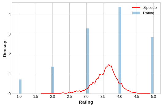
The distribution of the encoded Zipcode feature roughly follows the distribution of the actual ratings, meaning that movie-watchers differed enough in their ratings from zipcode to zipcode that our target encoding was able to capture useful information.
Exercise
0) 准备工作
import matplotlib.pyplot as plt
import numpy as np
import pandas as pd
import seaborn as sns
import warnings
from category_encoders import MEstimateEncoder
from sklearn.model_selection import cross_val_score
from xgboost import XGBRegressor

# Set Matplotlib defaults
plt.style.use("seaborn-whitegrid")
plt.rc("figure", autolayout=True)
plt.rc(
    "axes",
    labelweight="bold",
    labelsize="large",
    titleweight="bold",
    titlesize=14,
    titlepad=10,
)
warnings.filterwarnings('ignore')


def score_dataset(X, y, model=XGBRegressor()):
    # Label encoding for categoricals
    for colname in X.select_dtypes(["category", "object"]):
        X[colname], _ = X[colname].factorize()
    # Metric for Housing competition is RMSLE (Root Mean Squared Log Error)
    score = cross_val_score(
        model, X, y, cv=5, scoring="neg_mean_squared_log_error",
    )
    score = -1 * score.mean()
    score = np.sqrt(score)
    return score


df = pd.read_csv("../input/fe-course-data/ames.csv")
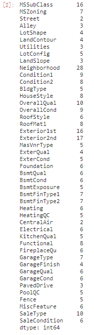
1) Choose Features for Encoding
First you’ll need to choose which features you want to apply a target encoding to. Categorical features with a large number of categories are often good candidates. Run this cell to see how many categories each categorical feature in the Ames dataset has.
df.select_dtypes(["object"]).nunique()
We talked about how the M-estimate encoding uses smoothing to improve estimates for rare categories. To see how many times a category occurs in the dataset, you can use the value_counts method. This cell shows the counts for SaleType, but you might want to consider others as well.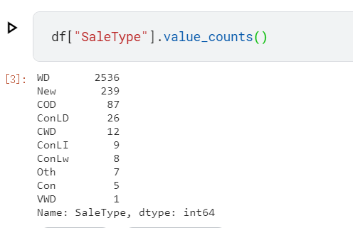
The Neighborhood feature looks promising. It has the most categories of any feature, and several categories are rare. Others that could be worth considering are SaleType,MSSubClass,Exterior1st,Exterior2nd. In fact, almost any of the nominal features would be worth trying because of the prevalence of rare categories.
2) Apply M-Estimate Encoding
from category_encoders import MEstimateEncoder
# Choose a set of features to encode and a value for m
encoder = MEstimateEncoder(cols=["Neighborhood"], m=5.0)


# Fit the encoder on the encoding split
encoder.fit(X_encode, y_encode)

# Encode the training split
X_train = encoder.transform(X_pretrain, y_train)


# Check your answer
q_2.check()
If you’d like to see how the encoded feature compares to the target, you can run this cell:
feature = encoder.cols

plt.figure(dpi=90)
ax = sns.distplot(y_train, kde=True, hist=False)
ax = sns.distplot(X_train[feature], color='r', ax=ax, hist=True, kde=False, norm_hist=True)
ax.set_xlabel("SalePrice");
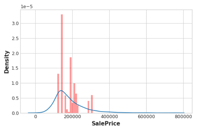
From the distribution plots, does it seem like the encoding is informative?
And this cell will show you the score of the encoded set compared to the original set:
X = df.copy()
y = X.pop("SalePrice")
score_base = score_dataset(X, y)
score_new = score_dataset(X_train, y_train)

print(f"Baseline Score: {score_base:.4f} RMSLE")
print(f"Score with Encoding: {score_new:.4f} RMSLE")
Baseline Score: 0.1428
RMSLE Score with Encoding: 0.1383 RMSLE
In this question, you’ll explore the problem of overfitting with target encodings. This will illustrate this importance of training fitting target encoders on data held-out from the training set.
So let’s see what happens when we fit the encoder and the model on the same dataset. To emphasize how dramatic the overfitting can be, we’ll mean-encode a feature that should have no relationship with SalePrice, a count:0, 1, 2, 3, 4, 5, ....
# Try experimenting with the smoothing parameter m
# Try 0, 1, 5, 50
m = 5

X = df.copy()
y = X.pop('SalePrice')

# Create an uninformative feature
X["Count"] = range(len(X))
X["Count"][1] = 0  # actually need one duplicate value to circumvent绕过 error-checking in MEstimateEncoder

# fit and transform on the same dataset
encoder = MEstimateEncoder(cols="Count", m=m)
X = encoder.fit_transform(X, y)

# Results
score =  score_dataset(X, y)
print(f"Score: {score:.4f} RMSLE")
Score: 0.0291 RMSLE
Almost a perfect score!
plt.figure(dpi=90)
ax = sns.distplot(y, kde=True, hist=False)
ax = sns.distplot(X["Count"], color='r', ax=ax, hist=True, kde=False, norm_hist=True)
ax.set_xlabel("SalePrice");
And the distributions are almost exactly the same, too.
3) Overfitting with Target Encoders
Since Count never has any duplicate values, the mean-encoded Count is essentially an exact copy of the target. In other words, mean-encoding turned a completely meaningless feature into a perfect feature.
Now, the only reason this worked is because we trained XGBoost on the same set we used to train the encoder. If we had used a hold-out set instead, none of this “fake” encoding would have transferred to the training data.
The lesson is that when using a target encoder it’s very important to use separate data sets for training the encoder and training the model. Otherwise the results can be very disappointing!
参考文献
Here are some great resources you might like to consult for more information.
They all played a part in shaping this course:
- The Art of Feature Engineering, a book by Pablo Duboue.
- An Empirical Analysis of Feature Engineering for Predictive Modeling, an article by Jeff Heaton.
- Feature Engineering for Machine Learning, a book by Alice Zheng and Amanda Casari. The tutorial on clustering was inspired by this excellent book.
- Feature Engineering and Selection, a book by Max Kuhn and Kjell Johnson.
Feature Engineering for House Prices
Data Preprocessing
Load Data
Establish Baseline
Step 2 - Feature Utility Scores
Step 3 - Create Features
k-Means Clustering
Principal Component Analysis
Target Encoding
Create Final Feature Set
Step 4 - Hyperparameter Tuning
Step 5 - Train Model And Create Submissions
Next Steps

若有收获,就点个赞吧
0 人点赞
