原文链接:https://blog.csdn.net/weixin_44791964/article/details/106533581?>
做一个 TF2…… 和 Keras 挺像的!

YOLOV4 是 YOLOV3 的改进版,在 YOLOV3 的基础上结合了非常多的小 Tricks。
尽管没有目标检测上革命性的改变,但是 YOLOV4 依然很好的结合了速度与精度。
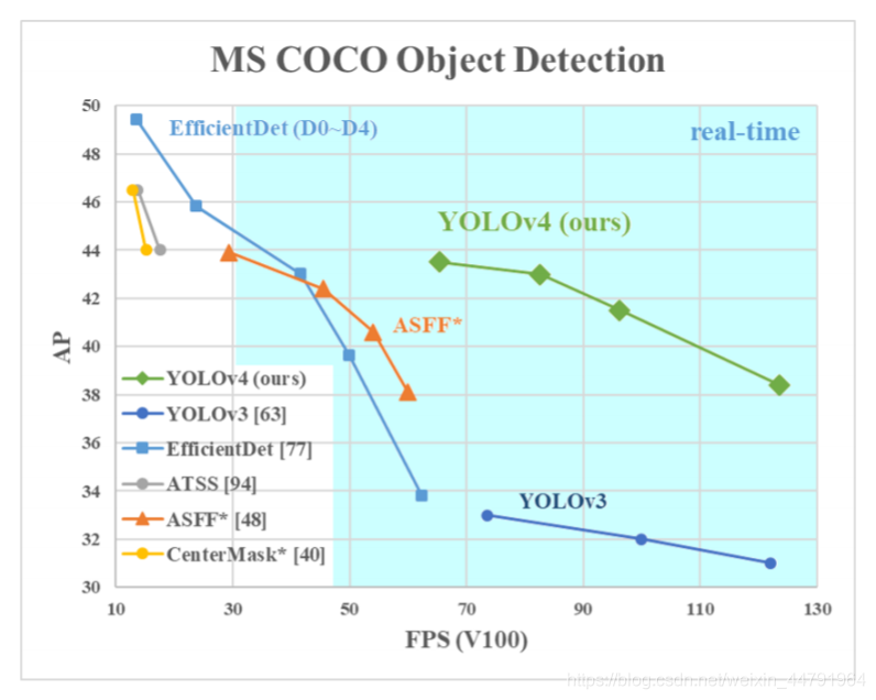
根据上图也可以看出来,YOLOV4 在 YOLOV3 的基础上,在 FPS 不下降的情况下,mAP 达到了 44,提高非常明显。
YOLOV4 整体上的检测思路和 YOLOV3 相比相差并不大,都是使用三个特征层进行分类与回归预测。
请注意!
强烈建议在学习 YOLOV4 之前学习 YOLOV3,因为 YOLOV4 确实可以看作是 YOLOV3 结合一系列改进的版本!
强烈建议在学习 YOLOV4 之前学习 YOLOV3,因为 YOLOV4 确实可以看作是 YOLOV3 结合一系列改进的版本!
强烈建议在学习 YOLOV4 之前学习 YOLOV3,因为 YOLOV4 确实可以看作是 YOLOV3 结合一系列改进的版本!
(重要的事情说三遍!)
YOLOV3 可参考该博客:
https://blog.csdn.net/weixin_44791964/article/details/103276106
https://github.com/bubbliiiing/yolov4-tf2
喜欢的可以给个 star 噢!
1、主干特征提取网络:DarkNet53 => CSPDarkNet53
2、特征金字塔:SPP,PAN
3、分类回归层:YOLOv3(未改变)
4、训练用到的小技巧:Mosaic 数据增强、Label Smoothing 平滑、CIOU、学习率余弦退火衰减
5、激活函数:使用 Mish 激活函数
以上并非全部的改进部分,还存在一些其它的改进,由于 YOLOV4 使用的改进实在太多了,很难完全实现与列出来,这里只列出来了一些我比较感兴趣,而且非常有效的改进。
整篇 BLOG 会结合 YOLOV3 与 YOLOV4 的差别进行解析
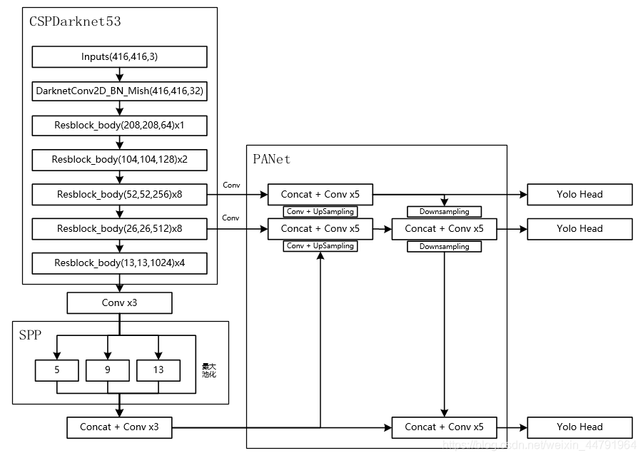
1、主干特征提取网络 Backbone
当输入是 416x416 时,特征结构如下:
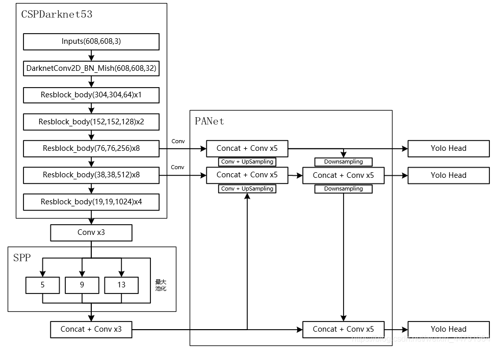
当输入是 608x608 时,特征结构如下:
主干特征提取网络 Backbone 的改进点有两个:
a). 主干特征提取网络:DarkNet53 => CSPDarkNet53
b). 激活函数:使用 Mish 激活函数
如果大家对 YOLOV3 比较熟悉的话,应该知道 Darknet53 的结构,其由一系列残差网络结构构成。在 Darknet53 中,其存在如下resblock_body 模块,其由一次下采样和多次残差结构的堆叠构成,Darknet53 便是由resblock_body 模块组合而成。
def resblock_body(x, num_filters, num_blocks):x = ZeroPadding2D(((1,0),(1,0)))(x)x = DarknetConv2D_BN_Leaky(num_filters, (3,3), strides=(2,2))(x)for i in range(num_blocks):y = DarknetConv2D_BN_Leaky(num_filters//2, (1,1))(x)y = DarknetConv2D_BN_Leaky(num_filters, (3,3))(y)x = Add()([x,y])return x
而在 YOLOV4 中,其对该部分进行了一定的修改。
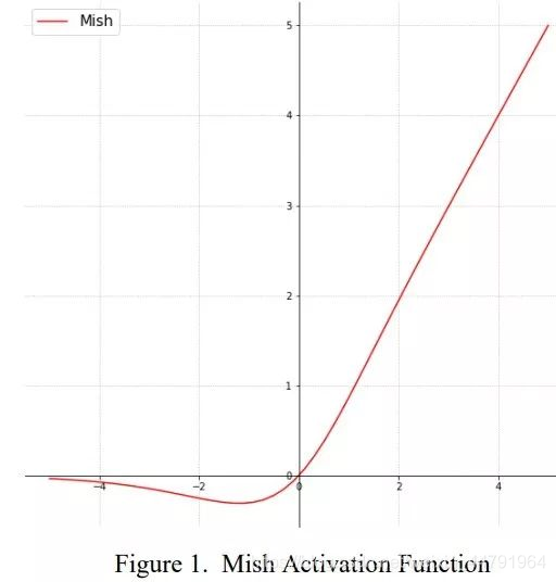
1、其一是将 DarknetConv2D 的激活函数由 LeakyReLU 修改成了 Mish,卷积块由DarknetConv2D_BN_Leaky 变成了 DarknetConv2D_BN_Mish。
Mish 函数的公式与图像如下:
Mish=x×tanh(ln(1+ex)) Mish=x \times tanh(ln(1+e^x))
2、其二是将 resblock_body 的结构进行修改,使用了 CSPnet 结构。此时 YOLOV4 当中的 Darknet53 被修改成了 CSPDarknet53。
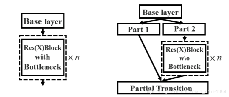
CSPnet 结构并不算复杂,就是将原来的残差块的堆叠进行了一个拆分,拆成左右两部分:
主干部分继续进行原来的残差块的堆叠;
另一部分则像一个残差边一样,经过少量处理直接连接到最后。
因此可以认为CSP 中存在一个大的残差边。
def resblock_body(x, num_filters, num_blocks, all_narrow=True):preconv1 = ZeroPadding2D(((1,0),(1,0)))(x)preconv1 = DarknetConv2D_BN_Mish(num_filters, (3,3), strides=(2,2))(preconv1)shortconv = DarknetConv2D_BN_Mish(num_filters//2 if all_narrow else num_filters, (1,1))(preconv1)mainconv = DarknetConv2D_BN_Mish(num_filters//2 if all_narrow else num_filters, (1,1))(preconv1)for i in range(num_blocks):y = compose(DarknetConv2D_BN_Mish(num_filters//2, (1,1)),DarknetConv2D_BN_Mish(num_filters//2 if all_narrow else num_filters, (3,3)))(mainconv)mainconv = Add()([mainconv,y])postconv = DarknetConv2D_BN_Mish(num_filters//2 if all_narrow else num_filters, (1,1))(mainconv)route = Concatenate()([postconv, shortconv])return DarknetConv2D_BN_Mish(num_filters, (1,1))(route)
全部实现代码为:
from functools import wrapsfrom tensorflow.keras import backend as Kfrom tensorflow.keras.layers import Conv2D, Add, ZeroPadding2D, UpSampling2D, Concatenate, MaxPooling2D, Layer, LeakyReLU, BatchNormalizationfrom tensorflow.keras.regularizers import l2from utils.utils import composeclass Mish(Layer):def __init__(self, **kwargs):super(Mish, self).__init__(**kwargs)self.supports_masking = Truedef call(self, inputs):return inputs * K.tanh(K.softplus(inputs))def get_config(self):config = super(Mish, self).get_config()return configdef compute_output_shape(self, input_shape):return input_shape@wraps(Conv2D)def DarknetConv2D(*args, **kwargs):darknet_conv_kwargs = {'kernel_regularizer': l2(5e-4)}darknet_conv_kwargs['padding'] = 'valid' if kwargs.get('strides')==(2,2) else 'same'darknet_conv_kwargs.update(kwargs)return Conv2D(*args, **darknet_conv_kwargs)def DarknetConv2D_BN_Mish(*args, **kwargs):no_bias_kwargs = {'use_bias': False}no_bias_kwargs.update(kwargs)return compose(DarknetConv2D(*args, **no_bias_kwargs),BatchNormalization(),Mish())def resblock_body(x, num_filters, num_blocks, all_narrow=True):preconv1 = ZeroPadding2D(((1,0),(1,0)))(x)preconv1 = DarknetConv2D_BN_Mish(num_filters, (3,3), strides=(2,2))(preconv1)shortconv = DarknetConv2D_BN_Mish(num_filters//2 if all_narrow else num_filters, (1,1))(preconv1)mainconv = DarknetConv2D_BN_Mish(num_filters//2 if all_narrow else num_filters, (1,1))(preconv1)for i in range(num_blocks):y = compose(DarknetConv2D_BN_Mish(num_filters//2, (1,1)),DarknetConv2D_BN_Mish(num_filters//2 if all_narrow else num_filters, (3,3)))(mainconv)mainconv = Add()([mainconv,y])postconv = DarknetConv2D_BN_Mish(num_filters//2 if all_narrow else num_filters, (1,1))(mainconv)route = Concatenate()([postconv, shortconv])return DarknetConv2D_BN_Mish(num_filters, (1,1))(route)def darknet_body(x):x = DarknetConv2D_BN_Mish(32, (3,3))(x)x = resblock_body(x, 64, 1, False)x = resblock_body(x, 128, 2)x = resblock_body(x, 256, 8)feat1 = xx = resblock_body(x, 512, 8)feat2 = xx = resblock_body(x, 1024, 4)feat3 = xreturn feat1,feat2,feat3
2、特征金字塔
当输入是 416x416 时,特征结构如下:
当输入是 608x608 时,特征结构如下:
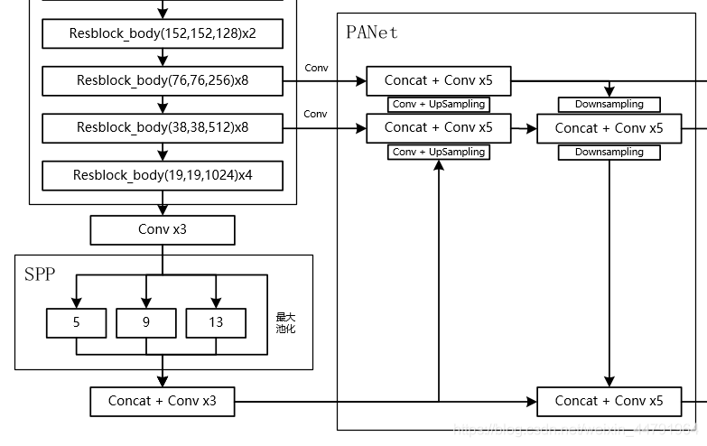
在特征金字塔部分,YOLOV4 结合了两种改进:
a). 使用了 SPP 结构。
b). 使用了 PANet 结构。
如上图所示,除去 CSPDarknet53 和 Yolo Head 的结构外,都是特征金字塔的结构。
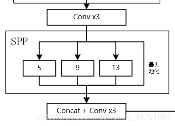
1、SPP 结构参杂在对 CSPdarknet53 的最后一个特征层的卷积里,在对 CSPdarknet53 的最后一个特征层进行三次 DarknetConv2D_BN_Leaky 卷积后,分别利用四个不同尺度的最大池化进行处理,最大池化的池化核大小分别为 13x13、9x9、5x5、1x1(1x1 即无处理)
maxpool1 = MaxPooling2D(pool_size=(13,13), strides=(1,1), padding='same')(P5)maxpool2 = MaxPooling2D(pool_size=(9,9), strides=(1,1), padding='same')(P5)maxpool3 = MaxPooling2D(pool_size=(5,5), strides=(1,1), padding='same')(P5)P5 = Concatenate()([maxpool1, maxpool2, maxpool3, P5])
其可以它能够极大地增加感受野,分离出最显著的上下文特征。
2、PANet 是 2018 的一种实例分割算法,其具体结构由反复提升特征的意思。
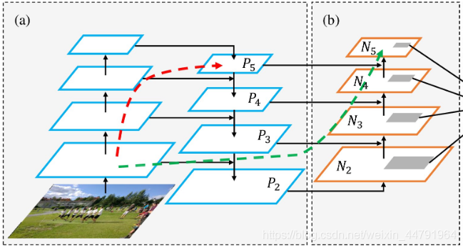
上图为原始的 PANet 的结构,可以看出来其具有一个非常重要的特点就是特征的反复提取。
在(a)里面是传统的特征金字塔结构,在完成特征金字塔从下到上的特征提取后,还需要实现(b)中从上到下的特征提取。
而在 YOLOV4 当中,其主要是在三个有效特征层上使用了 PANet 结构。
实现代码如下:
def yolo_body(inputs, num_anchors, num_classes):feat1,feat2,feat3 = darknet_body(inputs)P5 = DarknetConv2D_BN_Leaky(512, (1,1))(feat3)P5 = DarknetConv2D_BN_Leaky(1024, (3,3))(P5)P5 = DarknetConv2D_BN_Leaky(512, (1,1))(P5)maxpool1 = MaxPooling2D(pool_size=(13,13), strides=(1,1), padding='same')(P5)maxpool2 = MaxPooling2D(pool_size=(9,9), strides=(1,1), padding='same')(P5)maxpool3 = MaxPooling2D(pool_size=(5,5), strides=(1,1), padding='same')(P5)P5 = Concatenate()([maxpool1, maxpool2, maxpool3, P5])P5 = DarknetConv2D_BN_Leaky(512, (1,1))(P5)P5 = DarknetConv2D_BN_Leaky(1024, (3,3))(P5)P5 = DarknetConv2D_BN_Leaky(512, (1,1))(P5)P5_upsample = compose(DarknetConv2D_BN_Leaky(256, (1,1)), UpSampling2D(2))(P5)P4 = DarknetConv2D_BN_Leaky(256, (1,1))(feat2)P4 = Concatenate()([P4, P5_upsample])P4 = make_five_convs(P4,256)P4_upsample = compose(DarknetConv2D_BN_Leaky(128, (1,1)), UpSampling2D(2))(P4)P3 = DarknetConv2D_BN_Leaky(128, (1,1))(feat1)P3 = Concatenate()([P3, P4_upsample])P3 = make_five_convs(P3,128)P3_output = DarknetConv2D_BN_Leaky(256, (3,3))(P3)P3_output = DarknetConv2D(num_anchors*(num_classes+5), (1,1))(P3_output)P3_downsample = ZeroPadding2D(((1,0),(1,0)))(P3)P3_downsample = DarknetConv2D_BN_Leaky(256, (3,3), strides=(2,2))(P3_downsample)P4 = Concatenate()([P3_downsample, P4])P4 = make_five_convs(P4,256)P4_output = DarknetConv2D_BN_Leaky(512, (3,3))(P4)P4_output = DarknetConv2D(num_anchors*(num_classes+5), (1,1))(P4_output)P4_downsample = ZeroPadding2D(((1,0),(1,0)))(P4)P4_downsample = DarknetConv2D_BN_Leaky(512, (3,3), strides=(2,2))(P4_downsample)P5 = Concatenate()([P4_downsample, P5])P5 = make_five_convs(P5,512)P5_output = DarknetConv2D_BN_Leaky(1024, (3,3))(P5)P5_output = DarknetConv2D(num_anchors*(num_classes+5), (1,1))(P5_output)return Model(inputs, [P5_output, P4_output, P3_output])
3、YoloHead 利用获得到的特征进行预测
当输入是 416x416 时,特征结构如下:
当输入是 608x608 时,特征结构如下:
1、在特征利用部分,YoloV4 提取多特征层进行目标检测,一共提取三个特征层,分别位于中间层,中下层,底层,三个特征层的 shape 分别为 (76,76,256)、(38,38,512)、(19,19,1024)。
2、输出层的 shape 分别为 (19,19,75),(38,38,75),(76,76,75),最后一个维度为 75 是因为该图是基于 voc 数据集的,它的类为 20 种,YoloV4 只有针对每一个特征层存在 3 个先验框,所以最后维度为 3x25;
如果使用的是 coco 训练集,类则为 80 种,最后的维度应该为 255 = 3x85,三个特征层的 shape 为 (19,19,255),(38,38,255),(76,76,255)
实现代码如下:
def yolo_body(inputs, num_anchors, num_classes):P3_output = DarknetConv2D_BN_Leaky(256, (3,3))(P3)P3_output = DarknetConv2D(num_anchors*(num_classes+5), (1,1))(P3_output)P4_output = DarknetConv2D_BN_Leaky(512, (3,3))(P4)P4_output = DarknetConv2D(num_anchors*(num_classes+5), (1,1))(P4_output)P5_output = DarknetConv2D_BN_Leaky(1024, (3,3))(P5)P5_output = DarknetConv2D(num_anchors*(num_classes+5), (1,1))(P5_output)
4、预测结果的解码
由第二步我们可以获得三个特征层的预测结果,shape 分别为 (N,19,19,255),(N,38,38,255),(N,76,76,255) 的数据,对应每个图分为 19x19、38x38、76x76 的网格上 3 个预测框的位置。
但是这个预测结果并不对应着最终的预测框在图片上的位置,还需要解码才可以完成。
此处要讲一下 yolo3 的预测原理,yolo3 的 3 个特征层分别将整幅图分为 19x19、38x38、76x76 的网格,每个网络点负责一个区域的检测。
我们知道特征层的预测结果对应着三个预测框的位置,我们先将其 reshape 一下,其结果为 (N,19,19,3,85),(N,38,38,3,85),(N,76,76,3,85)。
最后一个维度中的 85 包含了 4+1+80,分别代表 x_offset、y_offset、h 和 w、置信度、分类结果。
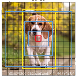
yolo3 的解码过程就是将每个网格点加上它对应的 x_offset 和 y_offset,加完后的结果就是预测框的中心,然后再利用 先验框和 h、w 结合 计算出预测框的长和宽。这样就能得到整个预测框的位置了。
当然得到最终的预测结构后还要进行得分排序与非极大抑制筛选
这一部分基本上是所有目标检测通用的部分。不过该项目的处理方式与其它项目不同。其对于每一个类进行判别。
1、取出每一类得分大于 self.obj_threshold 的框和得分。
2、利用框的位置和得分进行非极大抑制。
实现代码如下,当调用 yolo_eval 时,就会对每个特征层进行解码:
def yolo_head(feats, anchors, num_classes, input_shape, calc_loss=False):num_anchors = len(anchors)anchors_tensor = K.reshape(K.constant(anchors), [1, 1, 1, num_anchors, 2])grid_shape = K.shape(feats)[1:3]grid_y = K.tile(K.reshape(K.arange(0, stop=grid_shape[0]), [-1, 1, 1, 1]),[1, grid_shape[1], 1, 1])grid_x = K.tile(K.reshape(K.arange(0, stop=grid_shape[1]), [1, -1, 1, 1]),[grid_shape[0], 1, 1, 1])grid = K.concatenate([grid_x, grid_y])grid = K.cast(grid, K.dtype(feats))feats = K.reshape(feats, [-1, grid_shape[0], grid_shape[1], num_anchors, num_classes + 5])box_xy = (K.sigmoid(feats[..., :2]) + grid) / K.cast(grid_shape[::-1], K.dtype(feats))box_wh = K.exp(feats[..., 2:4]) * anchors_tensor / K.cast(input_shape[::-1], K.dtype(feats))box_confidence = K.sigmoid(feats[..., 4:5])box_class_probs = K.sigmoid(feats[..., 5:])if calc_loss == True:return grid, feats, box_xy, box_whreturn box_xy, box_wh, box_confidence, box_class_probsdef yolo_correct_boxes(box_xy, box_wh, input_shape, image_shape):box_yx = box_xy[..., ::-1]box_hw = box_wh[..., ::-1]input_shape = K.cast(input_shape, K.dtype(box_yx))image_shape = K.cast(image_shape, K.dtype(box_yx))new_shape = K.round(image_shape * K.min(input_shape/image_shape))offset = (input_shape-new_shape)/2./input_shapescale = input_shape/new_shapebox_yx = (box_yx - offset) * scalebox_hw *= scalebox_mins = box_yx - (box_hw / 2.)box_maxes = box_yx + (box_hw / 2.)boxes = K.concatenate([box_mins[..., 0:1],box_mins[..., 1:2],box_maxes[..., 0:1],box_maxes[..., 1:2]])boxes *= K.concatenate([image_shape, image_shape])return boxesdef yolo_boxes_and_scores(feats, anchors, num_classes, input_shape, image_shape):box_xy, box_wh, box_confidence, box_class_probs = yolo_head(feats, anchors, num_classes, input_shape)boxes = yolo_correct_boxes(box_xy, box_wh, input_shape, image_shape)boxes = K.reshape(boxes, [-1, 4])box_scores = box_confidence * box_class_probsbox_scores = K.reshape(box_scores, [-1, num_classes])return boxes, box_scoresdef yolo_eval(yolo_outputs,anchors,num_classes,image_shape,max_boxes=20,score_threshold=.6,iou_threshold=.5):num_layers = len(yolo_outputs)anchor_mask = [[6,7,8], [3,4,5], [0,1,2]]input_shape = K.shape(yolo_outputs[0])[1:3] * 32boxes = []box_scores = []for l in range(num_layers):_boxes, _box_scores = yolo_boxes_and_scores(yolo_outputs[l], anchors[anchor_mask[l]], num_classes, input_shape, image_shape)boxes.append(_boxes)box_scores.append(_box_scores)boxes = K.concatenate(boxes, axis=0)box_scores = K.concatenate(box_scores, axis=0)mask = box_scores >= score_thresholdmax_boxes_tensor = K.constant(max_boxes, dtype='int32')boxes_ = []scores_ = []classes_ = []for c in range(num_classes):class_boxes = tf.boolean_mask(boxes, mask[:, c])class_box_scores = tf.boolean_mask(box_scores[:, c], mask[:, c])nms_index = tf.image.non_max_suppression(class_boxes, class_box_scores, max_boxes_tensor, iou_threshold=iou_threshold)class_boxes = K.gather(class_boxes, nms_index)class_box_scores = K.gather(class_box_scores, nms_index)classes = K.ones_like(class_box_scores, 'int32') * cboxes_.append(class_boxes)scores_.append(class_box_scores)classes_.append(classes)boxes_ = K.concatenate(boxes_, axis=0)scores_ = K.concatenate(scores_, axis=0)classes_ = K.concatenate(classes_, axis=0)return boxes_, scores_, classes_
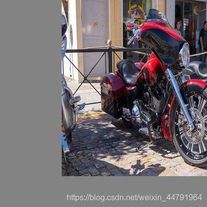
5、在原图上进行绘制
通过第四步,我们可以获得预测框在原图上的位置,而且这些预测框都是经过筛选的。这些筛选后的框可以直接绘制在图片上,就可以获得结果了。
1、YOLOV4 的改进训练技巧
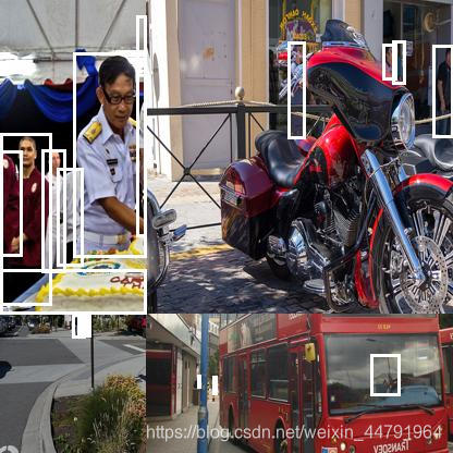
a)、Mosaic 数据增强
Yolov4 的 mosaic 数据增强参考了 CutMix 数据增强方式,理论上具有一定的相似性!
CutMix 数据增强方式利用两张图片进行拼接。
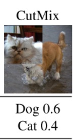
但是 mosaic 利用了四张图片,根据论文所说其拥有一个巨大的优点是丰富检测物体的背景!且在 BN 计算的时候一下子会计算四张图片的数据!
就像下图这样:
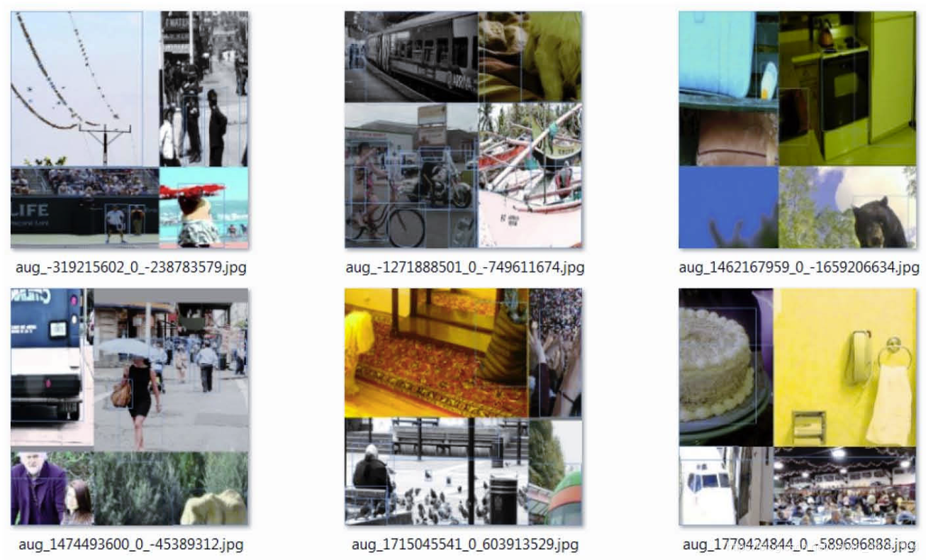
实现思路如下:
1、每次读取四张图片。

2、分别对四张图片进行翻转、缩放、色域变化等,并且按照四个方向位置摆好。

3、进行图片的组合和框的组合
def rand(a=0, b=1):return np.random.rand()*(b-a) + adef merge_bboxes(bboxes, cutx, cuty):merge_bbox = []for i in range(len(bboxes)):for box in bboxes[i]:tmp_box = []x1,y1,x2,y2 = box[0], box[1], box[2], box[3]if i == 0:if y1 > cuty or x1 > cutx:continueif y2 >= cuty and y1 <= cuty:y2 = cutyif y2-y1 < 5:continueif x2 >= cutx and x1 <= cutx:x2 = cutxif x2-x1 < 5:continueif i == 1:if y2 < cuty or x1 > cutx:continueif y2 >= cuty and y1 <= cuty:y1 = cutyif y2-y1 < 5:continueif x2 >= cutx and x1 <= cutx:x2 = cutxif x2-x1 < 5:continueif i == 2:if y2 < cuty or x2 < cutx:continueif y2 >= cuty and y1 <= cuty:y1 = cutyif y2-y1 < 5:continueif x2 >= cutx and x1 <= cutx:x1 = cutxif x2-x1 < 5:continueif i == 3:if y1 > cuty or x2 < cutx:continueif y2 >= cuty and y1 <= cuty:y2 = cutyif y2-y1 < 5:continueif x2 >= cutx and x1 <= cutx:x1 = cutxif x2-x1 < 5:continuetmp_box.append(x1)tmp_box.append(y1)tmp_box.append(x2)tmp_box.append(y2)tmp_box.append(box[-1])merge_bbox.append(tmp_box)return merge_bboxdef get_random_data(annotation_line, input_shape, random=True, hue=.1, sat=1.5, val=1.5, proc_img=True):'''random preprocessing for real-time data augmentation'''h, w = input_shapemin_offset_x = 0.4min_offset_y = 0.4scale_low = 1-min(min_offset_x,min_offset_y)scale_high = scale_low+0.2image_datas = []box_datas = []index = 0place_x = [0,0,int(w*min_offset_x),int(w*min_offset_x)]place_y = [0,int(h*min_offset_y),int(w*min_offset_y),0]for line in annotation_line:line_content = line.split()image = Image.open(line_content[0])image = image.convert("RGB")iw, ih = image.sizebox = np.array([np.array(list(map(int,box.split(',')))) for box in line_content[1:]])flip = rand()<.5if flip and len(box)>0:image = image.transpose(Image.FLIP_LEFT_RIGHT)box[:, [0,2]] = iw - box[:, [2,0]]new_ar = w/hscale = rand(scale_low, scale_high)if new_ar < 1:nh = int(scale*h)nw = int(nh*new_ar)else:nw = int(scale*w)nh = int(nw/new_ar)image = image.resize((nw,nh), Image.BICUBIC)hue = rand(-hue, hue)sat = rand(1, sat) if rand()<.5 else 1/rand(1, sat)val = rand(1, val) if rand()<.5 else 1/rand(1, val)x = rgb_to_hsv(np.array(image)/255.)x[..., 0] += huex[..., 0][x[..., 0]>1] -= 1x[..., 0][x[..., 0]<0] += 1x[..., 1] *= satx[..., 2] *= valx[x>1] = 1x[x<0] = 0image = hsv_to_rgb(x)image = Image.fromarray((image*255).astype(np.uint8))dx = place_x[index]dy = place_y[index]new_image = Image.new('RGB', (w,h), (128,128,128))new_image.paste(image, (dx, dy))image_data = np.array(new_image)/255index = index + 1box_data = []if len(box)>0:np.random.shuffle(box)box[:, [0,2]] = box[:, [0,2]]*nw/iw + dxbox[:, [1,3]] = box[:, [1,3]]*nh/ih + dybox[:, 0:2][box[:, 0:2]<0] = 0box[:, 2][box[:, 2]>w] = wbox[:, 3][box[:, 3]>h] = hbox_w = box[:, 2] - box[:, 0]box_h = box[:, 3] - box[:, 1]box = box[np.logical_and(box_w>1, box_h>1)]box_data = np.zeros((len(box),5))box_data[:len(box)] = boximage_datas.append(image_data)box_datas.append(box_data)img = Image.fromarray((image_data*255).astype(np.uint8))for j in range(len(box_data)):thickness = 3left, top, right, bottom = box_data[j][0:4]draw = ImageDraw.Draw(img)for i in range(thickness):draw.rectangle([left + i, top + i, right - i, bottom - i],outline=(255,255,255))img.show()cutx = np.random.randint(int(w*min_offset_x), int(w*(1 - min_offset_x)))cuty = np.random.randint(int(h*min_offset_y), int(h*(1 - min_offset_y)))new_image = np.zeros([h,w,3])new_image[:cuty, :cutx, :] = image_datas[0][:cuty, :cutx, :]new_image[cuty:, :cutx, :] = image_datas[1][cuty:, :cutx, :]new_image[cuty:, cutx:, :] = image_datas[2][cuty:, cutx:, :]new_image[:cuty, cutx:, :] = image_datas[3][:cuty, cutx:, :]new_boxes = merge_bboxes(box_datas, cutx, cuty)return new_image, new_boxes
b)、Label Smoothing 平滑
标签平滑的思想很简单,具体公式如下:
new_onehot_labels = onehot_labels * (1 - label_smoothing) + label_smoothing / num_classes
当 label_smoothing 的值为 0.01 得时候,公式变成如下所示:
new_onehot_labels = y * (1 - 0.01) + 0.01 / num_classes
其实 Label Smoothing 平滑就是将标签进行一个平滑,原始的标签是 0、1,在平滑后变成 0.005(如果是二分类)、0.995,也就是说对分类准确做了一点惩罚,让模型不可以分类的太准确,太准确容易过拟合。
实现代码如下:
def _smooth_labels(y_true, label_smoothing):num_classes = tf.cast(K.shape(y_true)[-1], dtype=K.floatx())label_smoothing = K.constant(label_smoothing, dtype=K.floatx())return y_true * (1.0 - label_smoothing) + label_smoothing / num_classes
c)、CIOU
IoU 是比值的概念,对目标物体的 scale 是不敏感的。然而常用的 BBox 的回归损失优化和 IoU 优化不是完全等价的,寻常的 IoU 无法直接优化没有重叠的部分。
于是有人提出直接使用 IOU 作为回归优化 loss,CIOU 是其中非常优秀的一种想法。
CIOU 将目标与 anchor 之间的距离,重叠率、尺度以及惩罚项都考虑进去,使得目标框回归变得更加稳定,不会像 IoU 和 GIoU 一样出现训练过程中发散等问题。而惩罚因子把预测框长宽比拟合目标框的长宽比考虑进去。
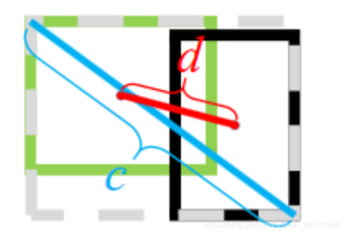
CIOU 公式如下
CIOU=IOU−ρ2(b,bgt)c2−αv CIOU = IOU - \frac{\rho{gt})}{c^2} - \alpha v
其中,ρ2(b,bgt) \rho{gt}) 分别代表了预测框和真实框的中心点的欧式距离。 c 代表的是能够同时包含预测框和真实框的最小闭包区域的对角线距离。
而α \alpha 和 v v 的公式如下
α=v1−IOU+v \alpha = \frac{v}{1-IOU+v}
v=4π2(arctanwgthgt−arctanwh)2 v = \frac{4}{\pi {gt}}{h2
把 1-CIOU 就可以得到相应的 LOSS 了。
LOSSCIOU=1−IOU+ρ2(b,bgt)c2+αv LOSS_{CIOU} = 1 - IOU + \frac{\rho{gt})}{c^2} + \alpha v
def box_ciou(b1, b2):"""输入为:----------b1: tensor, shape=(batch, feat_w, feat_h, anchor_num, 4), xywhb2: tensor, shape=(batch, feat_w, feat_h, anchor_num, 4), xywh返回为:-------ciou: tensor, shape=(batch, feat_w, feat_h, anchor_num, 1)"""b1_xy = b1[..., :2]b1_wh = b1[..., 2:4]b1_wh_half = b1_wh/2.b1_mins = b1_xy - b1_wh_halfb1_maxes = b1_xy + b1_wh_halfb2_xy = b2[..., :2]b2_wh = b2[..., 2:4]b2_wh_half = b2_wh/2.b2_mins = b2_xy - b2_wh_halfb2_maxes = b2_xy + b2_wh_halfintersect_mins = K.maximum(b1_mins, b2_mins)intersect_maxes = K.minimum(b1_maxes, b2_maxes)intersect_wh = K.maximum(intersect_maxes - intersect_mins, 0.)intersect_area = intersect_wh[..., 0] * intersect_wh[..., 1]b1_area = b1_wh[..., 0] * b1_wh[..., 1]b2_area = b2_wh[..., 0] * b2_wh[..., 1]union_area = b1_area + b2_area - intersect_areaiou = intersect_area / (union_area + K.epsilon())center_distance = K.sum(K.square(b1_xy - b2_xy), axis=-1)enclose_mins = K.minimum(b1_mins, b2_mins)enclose_maxes = K.maximum(b1_maxes, b2_maxes)enclose_wh = K.maximum(enclose_maxes - enclose_mins, 0.0)enclose_diagonal = K.sum(K.square(enclose_wh), axis=-1)ciou = iou - 1.0 * (center_distance) / (enclose_diagonal + K.epsilon())v = 4*K.square(tf.math.atan2(b1_wh[..., 0], b1_wh[..., 1]) - tf.math.atan2(b2_wh[..., 0], b2_wh[..., 1])) / (math.pi * math.pi)alpha = v / (1.0 - iou + v)ciou = ciou - alpha * vciou = K.expand_dims(ciou, -1)return ciou
d)、学习率余弦退火衰减
余弦退火衰减法,学习率会先上升再下降,这是退火优化法的思想。(关于什么是退火算法可以百度。)
上升的时候使用线性上升,下降的时候模拟 cos 函数下降。执行多次。
效果如图所示:
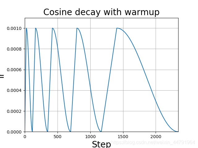
在 TF2 中可使用自带的 tf.keras.experimental.CosineDecayRestarts 实现。
余弦退火衰减有几个比较必要的参数:
1、learning_rate_base:学习率最高值。
2、first_decay_steps :多少充分一次。
lr_schedule = tf.keras.experimental.CosineDecayRestarts(initial_learning_rate = learning_rate_base,first_decay_steps = 5*epoch_size,t_mul = 1.0,alpha = 1e-2)optimizer = tf.keras.optimizers.Adam(learning_rate=lr_schedule)
2、loss 组成
a)、计算 loss 所需参数
在计算 loss 的时候,实际上是 y_pre 和 y_true 之间的对比:
y_pre 就是一幅图像经过网络之后的输出,内部含有三个特征层的内容;其需要解码才能够在图上作画
y_true 就是一个真实图像中,它的每个真实框对应的 (19,19)、(38,38)、(76,76) 网格上的偏移位置、长宽与种类。其仍需要编码才能与 y_pred 的结构一致
实际上 y_pre 和 y_true 内容的 shape 都是
(batch_size,19,19,3,85)
(batch_size,38,38,3,85)
(batch_size,76,76,3,85)
b)、y_pre 是什么
网络最后输出的内容就是三个特征层每个网格点对应的预测框及其种类,即三个特征层分别对应着图片被分为不同 size 的网格后,每个网格点上三个先验框对应的位置、置信度及其种类。
对于输出的 y1、y2、y3 而言,[…, : 2]指的是相对于每个网格点的偏移量,[…, 2: 4]指的是宽和高,[…, 4: 5]指的是该框的置信度,[…, 5: ]指的是每个种类的预测概率。
现在的 y_pre 还是没有解码的,解码了之后才是真实图像上的情况。
c)、y_true 是什么。
y_true 就是一个真实图像中,它的每个真实框对应的 (19,19)、(38,38)、(76,76) 网格上的偏移位置、长宽与种类。其仍需要编码才能与 y_pred 的结构一致
在 yolo4 中,其使用了一个专门的函数用于处理读取进来的图片的框的真实情况。
def preprocess_true_boxes(true_boxes, input_shape, anchors, num_classes):
其输入为:
true_boxes:shape 为 (m, T, 5) 代表 m 张图 T 个框的 x_min、y_min、x_max、y_max、class_id。
input_shape:输入的形状,此处为 608、608
anchors:代表 9 个先验框的大小
num_classes:种类的数量。
其实对真实框的处理是将真实框转化成图片中相对网格的 xyhw,步骤如下:
1、取框的真实值,获取其框的中心及其宽高,除去 input_shape 变成比例的模式。
2、建立全为 0 的 y_true,y_true 是一个列表,包含三个特征层,shape 分别为 (batch_size,19,19,3,85)、(batch_size,38,38,3,85)、(batch_size,76,76,3,85)。
3、对每一张图片处理,将每一张图片中的真实框的 wh 和先验框的 wh 对比,计算 IOU 值,选取其中 IOU 最高的一个,得到其所属特征层及其网格点的位置,在对应的 y_true 中将内容进行保存。
for t, n in enumerate(best_anchor):for l in range(num_layers):if n in anchor_mask[l]:i = np.floor(true_boxes[b,t,0]*grid_shapes[l][1]).astype('int32')j = np.floor(true_boxes[b,t,1]*grid_shapes[l][0]).astype('int32')k = anchor_mask[l].index(n)c = true_boxes[b,t, 4].astype('int32')y_true[l][b, j, i, k, 0:4] = true_boxes[b,t, 0:4]y_true[l][b, j, i, k, 4] = 1y_true[l][b, j, i, k, 5+c] = 1
对于最后输出的 y_true 而言,只有每个图里每个框最对应的位置有数据,其它的地方都为 0。
preprocess_true_boxes 全部的代码如下:
def preprocess_true_boxes(true_boxes, input_shape, anchors, num_classes):assert (true_boxes[..., 4]<num_classes).all(), 'class id must be less than num_classes'num_layers = len(anchors)//3anchor_mask = [[6,7,8], [3,4,5], [0,1,2]] if num_layers==3 else [[3,4,5], [1,2,3]]true_boxes = np.array(true_boxes, dtype='float32')input_shape = np.array(input_shape, dtype='int32')boxes_xy = (true_boxes[..., 0:2] + true_boxes[..., 2:4]) // 2boxes_wh = true_boxes[..., 2:4] - true_boxes[..., 0:2]true_boxes[..., 0:2] = boxes_xy/input_shape[:]true_boxes[..., 2:4] = boxes_wh/input_shape[:]m = true_boxes.shape[0]grid_shapes = [input_shape//{0:32, 1:16, 2:8}[l] for l in range(num_layers)]y_true = [np.zeros((m,grid_shapes[l][0],grid_shapes[l][1],len(anchor_mask[l]),5+num_classes),dtype='float32') for l in range(num_layers)]anchors = np.expand_dims(anchors, 0)anchor_maxes = anchors / 2.anchor_mins = -anchor_maxesvalid_mask = boxes_wh[..., 0]>0for b in range(m):wh = boxes_wh[b, valid_mask[b]]if len(wh)==0: continuewh = np.expand_dims(wh, -2)box_maxes = wh / 2.box_mins = -box_maxesintersect_mins = np.maximum(box_mins, anchor_mins)intersect_maxes = np.minimum(box_maxes, anchor_maxes)intersect_wh = np.maximum(intersect_maxes - intersect_mins, 0.)intersect_area = intersect_wh[..., 0] * intersect_wh[..., 1]box_area = wh[..., 0] * wh[..., 1]anchor_area = anchors[..., 0] * anchors[..., 1]iou = intersect_area / (box_area + anchor_area - intersect_area)best_anchor = np.argmax(iou, axis=-1)for t, n in enumerate(best_anchor):for l in range(num_layers):if n in anchor_mask[l]:i = np.floor(true_boxes[b,t,0]*grid_shapes[l][1]).astype('int32')j = np.floor(true_boxes[b,t,1]*grid_shapes[l][0]).astype('int32')k = anchor_mask[l].index(n)c = true_boxes[b,t, 4].astype('int32')y_true[l][b, j, i, k, 0:4] = true_boxes[b,t, 0:4]y_true[l][b, j, i, k, 4] = 1y_true[l][b, j, i, k, 5+c] = 1return y_true
d)、loss 的计算过程
在得到了 y_pre 和 y_true 后怎么对比呢?不是简单的减一下!
loss 值需要对三个特征层进行处理,这里以最小的特征层为例。
1、利用 y_true 取出该特征层中真实存在目标的点的位置 (m,19,19,3,1) 及其对应的种类(m,19,19,3,80)。
2、将 yolo_outputs 的预测值输出进行处理,得到 reshape 后的预测值 y_pre,shape 为 (m,19,19,3,85)。还有解码后的 xy,wh。
3、对于每一幅图,计算其中所有真实框与预测框的 IOU,如果某些预测框和真实框的重合程度大于 0.5,则忽略。
4、计算 ciou 作为回归的 loss,这里只计算正样本的回归 loss。
5、计算置信度的 loss,其有两部分构成,第一部分是实际上存在目标的,预测结果中置信度的值与 1 对比;第二部分是实际上不存在目标的,预测结果中置信度的值与 0 对比。
6、计算预测种类的 loss,其计算的是实际上存在目标的,预测类与真实类的差距。
其实际上计算的总的 loss 是三个 loss 的和,这三个 loss 分别是:
- 实际存在的框,CIOU LOSS。
- 实际存在的框,预测结果中置信度的值与 1 对比;实际不存在的框,预测结果中置信度的值与 0 对比,该部分要去除被忽略的不包含目标的框。
- 实际存在的框,种类预测结果与实际结果的对比。
其实际代码如下,使用 yolo_loss 就可以获得 loss 值:
def _smooth_labels(y_true, label_smoothing):num_classes = K.shape(y_true)[-1],label_smoothing = K.constant(label_smoothing, dtype=K.floatx())return y_true * (1.0 - label_smoothing) + label_smoothing / num_classesdef yolo_head(feats, anchors, num_classes, input_shape, calc_loss=False):num_anchors = len(anchors)anchors_tensor = K.reshape(K.constant(anchors), [1, 1, 1, num_anchors, 2])grid_shape = K.shape(feats)[1:3]grid_y = K.tile(K.reshape(K.arange(0, stop=grid_shape[0]), [-1, 1, 1, 1]),[1, grid_shape[1], 1, 1])grid_x = K.tile(K.reshape(K.arange(0, stop=grid_shape[1]), [1, -1, 1, 1]),[grid_shape[0], 1, 1, 1])grid = K.concatenate([grid_x, grid_y])grid = K.cast(grid, K.dtype(feats))feats = K.reshape(feats, [-1, grid_shape[0], grid_shape[1], num_anchors, num_classes + 5])box_xy = (K.sigmoid(feats[..., :2]) + grid) / K.cast(grid_shape[::-1], K.dtype(feats))box_wh = K.exp(feats[..., 2:4]) * anchors_tensor / K.cast(input_shape[::-1], K.dtype(feats))box_confidence = K.sigmoid(feats[..., 4:5])box_class_probs = K.sigmoid(feats[..., 5:])if calc_loss == True:return grid, feats, box_xy, box_whreturn box_xy, box_wh, box_confidence, box_class_probsdef box_iou(b1, b2):b1 = K.expand_dims(b1, -2)b1_xy = b1[..., :2]b1_wh = b1[..., 2:4]b1_wh_half = b1_wh/2.b1_mins = b1_xy - b1_wh_halfb1_maxes = b1_xy + b1_wh_halfb2 = K.expand_dims(b2, 0)b2_xy = b2[..., :2]b2_wh = b2[..., 2:4]b2_wh_half = b2_wh/2.b2_mins = b2_xy - b2_wh_halfb2_maxes = b2_xy + b2_wh_halfintersect_mins = K.maximum(b1_mins, b2_mins)intersect_maxes = K.minimum(b1_maxes, b2_maxes)intersect_wh = K.maximum(intersect_maxes - intersect_mins, 0.)intersect_area = intersect_wh[..., 0] * intersect_wh[..., 1]b1_area = b1_wh[..., 0] * b1_wh[..., 1]b2_area = b2_wh[..., 0] * b2_wh[..., 1]iou = intersect_area / (b1_area + b2_area - intersect_area)return ioudef yolo_loss(args, anchors, num_classes, ignore_thresh=.5, label_smoothing=0.1, print_loss=False):num_layers = len(anchors)//3y_true = args[num_layers:]yolo_outputs = args[:num_layers]anchor_mask = [[6,7,8], [3,4,5], [0,1,2]] if num_layers==3 else [[3,4,5], [1,2,3]]input_shape = K.cast(K.shape(yolo_outputs[0])[1:3] * 32, K.dtype(y_true[0]))loss = 0m = K.shape(yolo_outputs[0])[0]mf = K.cast(m, K.dtype(yolo_outputs[0]))for l in range(num_layers):object_mask = y_true[l][..., 4:5]true_class_probs = y_true[l][..., 5:]if label_smoothing:true_class_probs = _smooth_labels(true_class_probs, label_smoothing)grid, raw_pred, pred_xy, pred_wh = yolo_head(yolo_outputs[l],anchors[anchor_mask[l]], num_classes, input_shape, calc_loss=True)pred_box = K.concatenate([pred_xy, pred_wh])ignore_mask = tf.TensorArray(K.dtype(y_true[0]), size=1, dynamic_size=True)object_mask_bool = K.cast(object_mask, 'bool')def loop_body(b, ignore_mask):true_box = tf.boolean_mask(y_true[l][b,...,0:4], object_mask_bool[b,...,0])iou = box_iou(pred_box[b], true_box)best_iou = K.max(iou, axis=-1)ignore_mask = ignore_mask.write(b, K.cast(best_iou<ignore_thresh, K.dtype(true_box)))return b+1, ignore_mask_, ignore_mask = tf.while_loop(lambda b,*args: b<m, loop_body, [0, ignore_mask])ignore_mask = ignore_mask.stack()ignore_mask = K.expand_dims(ignore_mask, -1)box_loss_scale = 2 - y_true[l][...,2:3]*y_true[l][...,3:4]raw_true_box = y_true[l][...,0:4]ciou = box_ciou(pred_box, raw_true_box)ciou_loss = object_mask * box_loss_scale * (1 - ciou)ciou_loss = K.sum(ciou_loss) / mflocation_loss = ciou_lossconfidence_loss = object_mask * K.binary_crossentropy(object_mask, raw_pred[...,4:5], from_logits=True)+ \(1-object_mask) * K.binary_crossentropy(object_mask, raw_pred[...,4:5], from_logits=True) * ignore_maskclass_loss = object_mask * K.binary_crossentropy(true_class_probs, raw_pred[...,5:], from_logits=True)confidence_loss = K.sum(confidence_loss) / mfclass_loss = K.sum(class_loss) / mfloss += location_loss + confidence_loss + class_lossloss = K.expand_dims(loss, axis=-1)return loss
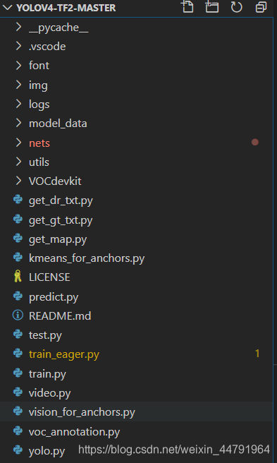
yolo4 整体的文件夹构架如下:
本文使用 VOC 格式进行训练。
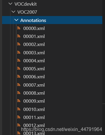
训练前将标签文件放在 VOCdevkit 文件夹下的 VOC2007 文件夹下的 Annotation 中。
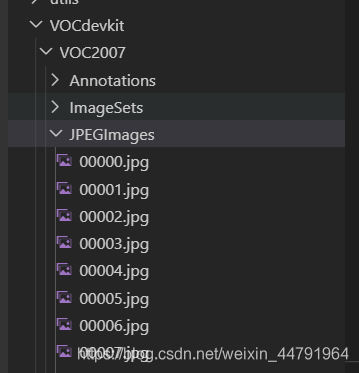
训练前将图片文件放在 VOCdevkit 文件夹下的 VOC2007 文件夹下的 JPEGImages 中。
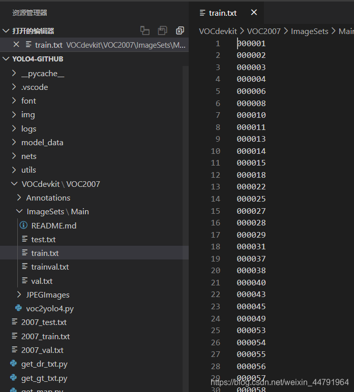
在训练前利用 voc2yolo4.py 文件生成对应的 txt。
再运行根目录下的 voc_annotation.py,运行前需要将 classes 改成你自己的 classes。
classes = ["aeroplane", "bicycle", "bird", "boat", "bottle", "bus", "car", "cat", "chair", "cow", "diningtable", "dog", "horse", "motorbike", "person", "pottedplant", "sheep", "sofa", "train", "tvmonitor"]
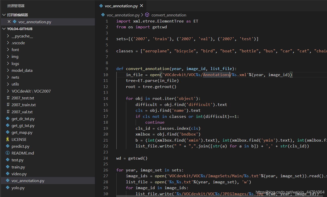
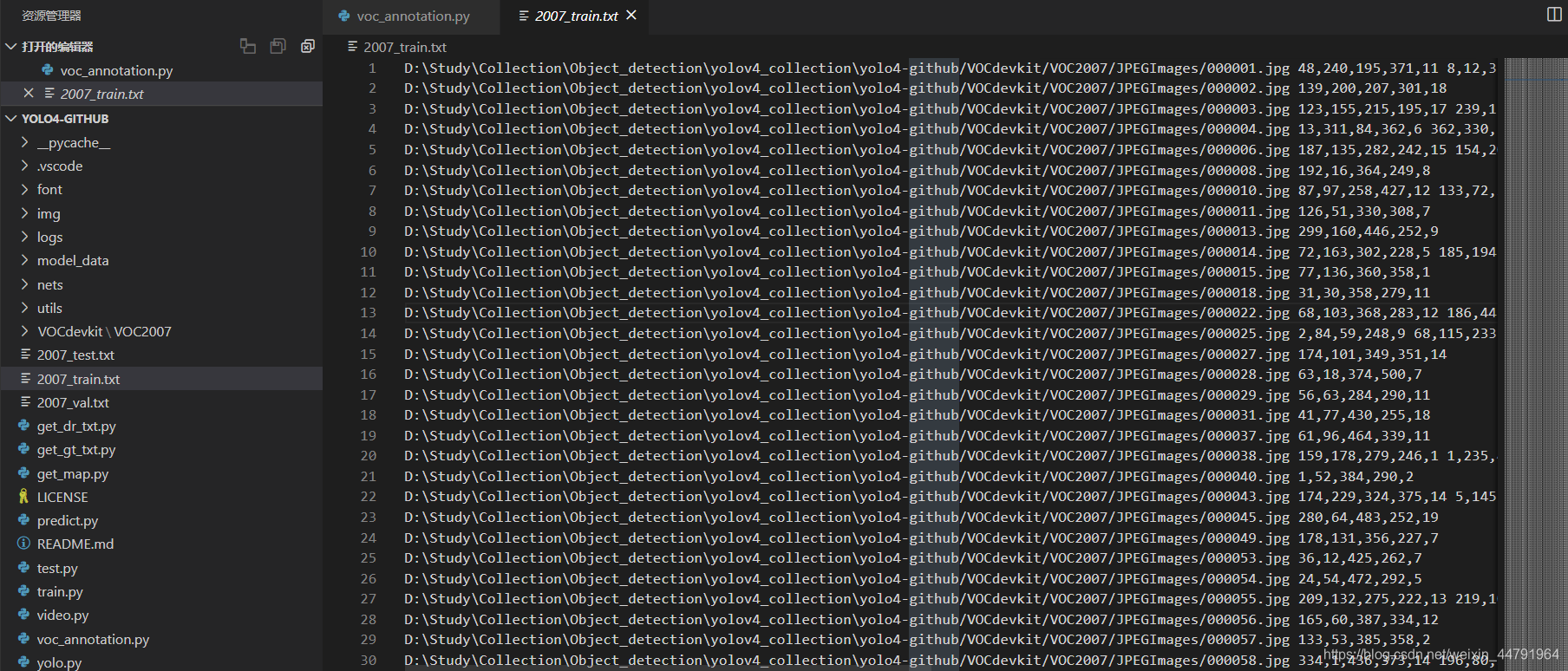
就会生成对应的 2007_train.txt,每一行对应其图片位置及其真实框的位置。
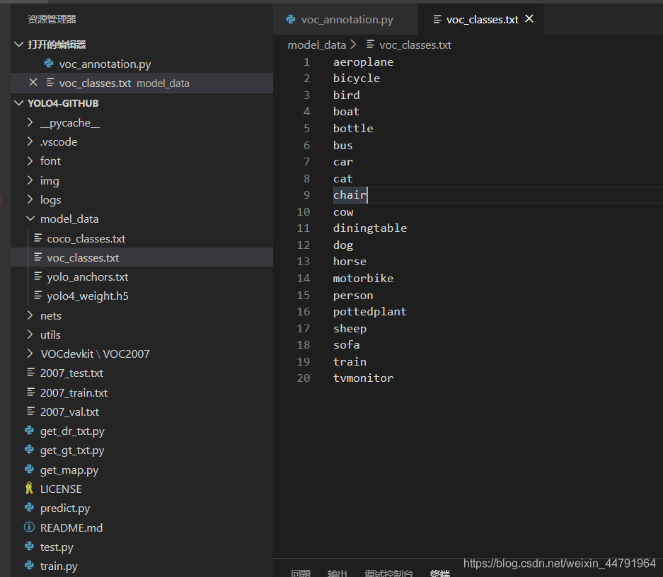
在训练前需要修改 model_data 里面的 voc_classes.txt 文件,需要将 classes 改成你自己的 classes。
运行 train.py 即可开始训练。

为了适配 Tensorflow2 的 Eager 模式,我也专门建立了一个 train_eager.py。其中参数与 train.py 差不多。也可以运行进行训练。
https://blog.csdn.net/weixin_44791964/article/details/106533581?>

若有收获,就点个赞吧
0 人点赞
