- Merge, join, and concatenate
- Concatenating objects
- Database-style DataFrame or named Series joining/merging
- Brief primer on merge methods (relational algebra)
- Checking for duplicate keys
- The merge indicator
- Merge dtypes
- Joining on index
- Joining key columns on an index
- Joining a single Index to a MultiIndex
- Joining with two MultiIndexes
- Merging on a combination of columns and index levels
- Overlapping value columns
- Joining multiple DataFrames
- Merging together values within Series or DataFrame columns
- Timeseries friendly merging
Merge, join, and concatenate
pandas provides various facilities for easily combining together Series or DataFrame with various kinds of set logic for the indexes and relational algebra functionality in the case of join / merge-type operations.
Concatenating objects
The concat() function (in the main pandas namespace) does all of
the heavy lifting of performing concatenation operations along an axis while
performing optional set logic (union or intersection) of the indexes (if any) on
the other axes. Note that I say “if any” because there is only a single possible
axis of concatenation for Series.
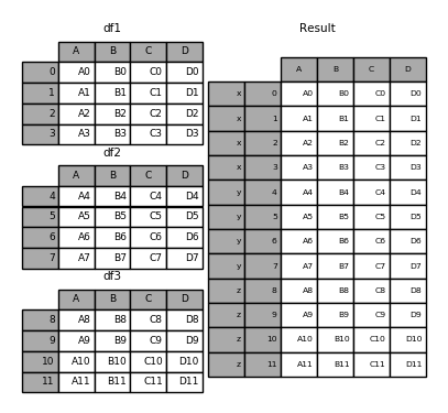
Before diving into all of the details of concat and what it can do, here is
a simple example:
In [1]: df1 = pd.DataFrame({'A': ['A0', 'A1', 'A2', 'A3'],...: 'B': ['B0', 'B1', 'B2', 'B3'],...: 'C': ['C0', 'C1', 'C2', 'C3'],...: 'D': ['D0', 'D1', 'D2', 'D3']},...: index=[0, 1, 2, 3])...:In [2]: df2 = pd.DataFrame({'A': ['A4', 'A5', 'A6', 'A7'],...: 'B': ['B4', 'B5', 'B6', 'B7'],...: 'C': ['C4', 'C5', 'C6', 'C7'],...: 'D': ['D4', 'D5', 'D6', 'D7']},...: index=[4, 5, 6, 7])...:In [3]: df3 = pd.DataFrame({'A': ['A8', 'A9', 'A10', 'A11'],...: 'B': ['B8', 'B9', 'B10', 'B11'],...: 'C': ['C8', 'C9', 'C10', 'C11'],...: 'D': ['D8', 'D9', 'D10', 'D11']},...: index=[8, 9, 10, 11])...:In [4]: frames = [df1, df2, df3]In [5]: result = pd.concat(frames)
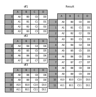
Like its sibling function on ndarrays, numpy.concatenate, pandas.concat
takes a list or dict of homogeneously-typed objects and concatenates them with
some configurable handling of “what to do with the other axes”:
pd.concat(objs, axis=0, join='outer', ignore_index=False, keys=None,levels=None, names=None, verify_integrity=False, copy=True)
objs: a sequence or mapping of Series or DataFrame objects. If a dict is passed, the sorted keys will be used as the keys argument, unless it is passed, in which case the values will be selected (see below). Any None objects will be dropped silently unless they are all None in which case a ValueError will be raised.axis: {0, 1, …}, default 0. The axis to concatenate along.join: {‘inner’, ‘outer’}, default ‘outer’. How to handle indexes on other axis(es). Outer for union and inner for intersection.ignore_index: boolean, default False. If True, do not use the index values on the concatenation axis. The resulting axis will be labeled 0, …, n - 1. This is useful if you are concatenating objects where the concatenation axis does not have meaningful indexing information. Note the index values on the other axes are still respected in the join.keys: sequence, default None. Construct hierarchical index using the passed keys as the outermost level. If multiple levels passed, should contain tuples.levels: list of sequences, default None. Specific levels (unique values) to use for constructing a MultiIndex. Otherwise they will be inferred from the keys.names: list, default None. Names for the levels in the resulting hierarchical index.verify_integrity: boolean, default False. Check whether the new concatenated axis contains duplicates. This can be very expensive relative to the actual data concatenation.copy: boolean, default True. If False, do not copy data unnecessarily.
Without a little bit of context many of these arguments don’t make much sense.
Let’s revisit the above example. Suppose we wanted to associate specific keys
with each of the pieces of the chopped up DataFrame. We can do this using the
keys argument:
In [6]: result = pd.concat(frames, keys=['x', 'y', 'z'])

As you can see (if you’ve read the rest of the documentation), the resulting object’s index has a hierarchical index. This means that we can now select out each chunk by key:
In [7]: result.loc['y']Out[7]:A B C D4 A4 B4 C4 D45 A5 B5 C5 D56 A6 B6 C6 D67 A7 B7 C7 D7
It’s not a stretch to see how this can be very useful. More detail on this functionality below.
::: tip Note
It is worth noting that concat() (and therefore
append()) makes a full copy of the data, and that constantly
reusing this function can create a significant performance hit. If you need
to use the operation over several datasets, use a list comprehension.
:::
frames = [ process_your_file(f) for f in files ]result = pd.concat(frames)
Set logic on the other axes
When gluing together multiple DataFrames, you have a choice of how to handle the other axes (other than the one being concatenated). This can be done in the following two ways:
- Take the union of them all,
join='outer'. This is the default option as it results in zero information loss. - Take the intersection,
join='inner'.
Here is an example of each of these methods. First, the default join='outer'
behavior:
In [8]: df4 = pd.DataFrame({'B': ['B2', 'B3', 'B6', 'B7'],...: 'D': ['D2', 'D3', 'D6', 'D7'],...: 'F': ['F2', 'F3', 'F6', 'F7']},...: index=[2, 3, 6, 7])...:In [9]: result = pd.concat([df1, df4], axis=1, sort=False)
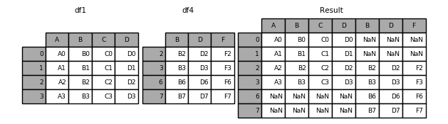
::: danger Warning
Changed in version 0.23.0.
The default behavior with join='outer' is to sort the other axis
(columns in this case). In a future version of pandas, the default will
be to not sort. We specified sort=False to opt in to the new
behavior now.
:::
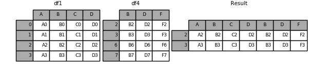
Here is the same thing with join='inner':
In [10]: result = pd.concat([df1, df4], axis=1, join='inner')
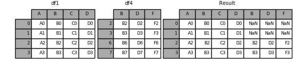
Lastly, suppose we just wanted to reuse the exact index from the original DataFrame:
In [11]: result = pd.concat([df1, df4], axis=1).reindex(df1.index)
Similarly, we could index before the concatenation:
In [12]: pd.concat([df1, df4.reindex(df1.index)], axis=1)Out[12]:A B C D B D F0 A0 B0 C0 D0 NaN NaN NaN1 A1 B1 C1 D1 NaN NaN NaN2 A2 B2 C2 D2 B2 D2 F23 A3 B3 C3 D3 B3 D3 F3
Concatenating using append
A useful shortcut to concat() are the append()
instance methods on Series and DataFrame. These methods actually predated
concat. They concatenate along axis=0, namely the index:
In [13]: result = df1.append(df2)
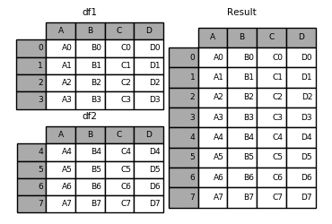
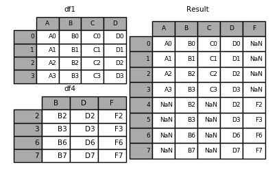
In the case of DataFrame, the indexes must be disjoint but the columns do not
need to be:
In [14]: result = df1.append(df4, sort=False)

append may take multiple objects to concatenate:
In [15]: result = df1.append([df2, df3])

::: tip Note
Unlike the append() method, which appends to the original list
and returns None, append() here does not modify
df1 and returns its copy with df2 appended.
:::
Ignoring indexes on the concatenation axis
For DataFrame objects which don’t have a meaningful index, you may wish
to append them and ignore the fact that they may have overlapping indexes. To
do this, use the ignore_index argument:
In [16]: result = pd.concat([df1, df4], ignore_index=True, sort=False)
This is also a valid argument to DataFrame.append():
In [17]: result = df1.append(df4, ignore_index=True, sort=False)

Concatenating with mixed ndims
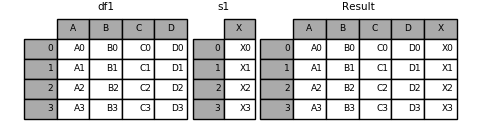
You can concatenate a mix of Series and DataFrame objects. The
Series will be transformed to DataFrame with the column name as
the name of the Series.
In [18]: s1 = pd.Series(['X0', 'X1', 'X2', 'X3'], name='X')In [19]: result = pd.concat([df1, s1], axis=1)
::: tip Note
Since we’re concatenating a Series to a DataFrame, we could have
achieved the same result with DataFrame.assign(). To concatenate an
arbitrary number of pandas objects (DataFrame or Series), use
concat.
:::
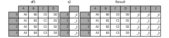
If unnamed Series are passed they will be numbered consecutively.
In [20]: s2 = pd.Series(['_0', '_1', '_2', '_3'])In [21]: result = pd.concat([df1, s2, s2, s2], axis=1)
Passing ignore_index=True will drop all name references.
In [22]: result = pd.concat([df1, s1], axis=1, ignore_index=True)

More concatenating with group keys
A fairly common use of the keys argument is to override the column names
when creating a new DataFrame based on existing Series.
Notice how the default behaviour consists on letting the resulting DataFrame
inherit the parent Series’ name, when these existed.
In [23]: s3 = pd.Series([0, 1, 2, 3], name='foo')In [24]: s4 = pd.Series([0, 1, 2, 3])In [25]: s5 = pd.Series([0, 1, 4, 5])In [26]: pd.concat([s3, s4, s5], axis=1)Out[26]:foo 0 10 0 0 01 1 1 12 2 2 43 3 3 5
Through the keys argument we can override the existing column names.
In [27]: pd.concat([s3, s4, s5], axis=1, keys=['red', 'blue', 'yellow'])Out[27]:red blue yellow0 0 0 01 1 1 12 2 2 43 3 3 5
Let’s consider a variation of the very first example presented:
In [28]: result = pd.concat(frames, keys=['x', 'y', 'z'])

You can also pass a dict to concat in which case the dict keys will be used
for the keys argument (unless other keys are specified):
In [29]: pieces = {'x': df1, 'y': df2, 'z': df3}In [30]: result = pd.concat(pieces)

In [31]: result = pd.concat(pieces, keys=['z', 'y'])

The MultiIndex created has levels that are constructed from the passed keys and
the index of the DataFrame pieces:
In [32]: result.index.levelsOut[32]: FrozenList([['z', 'y'], [4, 5, 6, 7, 8, 9, 10, 11]])
If you wish to specify other levels (as will occasionally be the case), you can
do so using the levels argument:
In [33]: result = pd.concat(pieces, keys=['x', 'y', 'z'],....: levels=[['z', 'y', 'x', 'w']],....: names=['group_key'])....:
In [34]: result.index.levelsOut[34]: FrozenList([['z', 'y', 'x', 'w'], [0, 1, 2, 3, 4, 5, 6, 7, 8, 9, 10, 11]])
This is fairly esoteric, but it is actually necessary for implementing things like GroupBy where the order of a categorical variable is meaningful.
Appending rows to a DataFrame
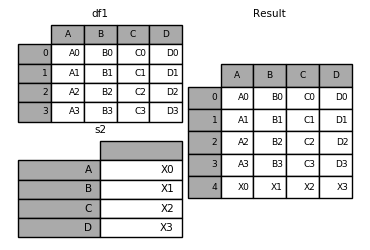
While not especially efficient (since a new object must be created), you can
append a single row to a DataFrame by passing a Series or dict to
append, which returns a new DataFrame as above.
In [35]: s2 = pd.Series(['X0', 'X1', 'X2', 'X3'], index=['A', 'B', 'C', 'D'])In [36]: result = df1.append(s2, ignore_index=True)
You should use ignore_index with this method to instruct DataFrame to
discard its index. If you wish to preserve the index, you should construct an
appropriately-indexed DataFrame and append or concatenate those objects.
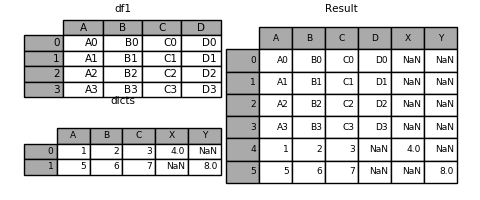
You can also pass a list of dicts or Series:
In [37]: dicts = [{'A': 1, 'B': 2, 'C': 3, 'X': 4},....: {'A': 5, 'B': 6, 'C': 7, 'Y': 8}]....:In [38]: result = df1.append(dicts, ignore_index=True, sort=False)
Database-style DataFrame or named Series joining/merging
pandas has full-featured, high performance in-memory join operations
idiomatically very similar to relational databases like SQL. These methods
perform significantly better (in some cases well over an order of magnitude
better) than other open source implementations (like base::merge.data.frame
in R). The reason for this is careful algorithmic design and the internal layout
of the data in DataFrame.
See the cookbook for some advanced strategies.
Users who are familiar with SQL but new to pandas might be interested in a comparison with SQL.
pandas provides a single function, merge(), as the entry point for
all standard database join operations between DataFrame or named Series objects:
pd.merge(left, right, how='inner', on=None, left_on=None, right_on=None,left_index=False, right_index=False, sort=True,suffixes=('_x', '_y'), copy=True, indicator=False,validate=None)
left: A DataFrame or named Series object.right: Another DataFrame or named Series object.on: Column or index level names to join on. Must be found in both the left and right DataFrame and/or Series objects. If not passed andleft_indexandright_indexareFalse, the intersection of the columns in the DataFrames and/or Series will be inferred to be the join keys.left_on: Columns or index levels from the left DataFrame or Series to use as keys. Can either be column names, index level names, or arrays with length equal to the length of the DataFrame or Series.right_on: Columns or index levels from the right DataFrame or Series to use as keys. Can either be column names, index level names, or arrays with length equal to the length of the DataFrame or Series.left_index: IfTrue, use the index (row labels) from the left DataFrame or Series as its join key(s). In the case of a DataFrame or Series with a MultiIndex (hierarchical), the number of levels must match the number of join keys from the right DataFrame or Series.right_index: Same usage asleft_indexfor the right DataFrame or Serieshow: One of'left','right','outer','inner'. Defaults toinner. See below for more detailed description of each method.sort: Sort the result DataFrame by the join keys in lexicographical order. Defaults toTrue, setting toFalsewill improve performance substantially in many cases.suffixes: A tuple of string suffixes to apply to overlapping columns. Defaults to('_x', '_y').copy: Always copy data (defaultTrue) from the passed DataFrame or named Series objects, even when reindexing is not necessary. Cannot be avoided in many cases but may improve performance / memory usage. The cases where copying can be avoided are somewhat pathological but this option is provided nonetheless.indicator: Add a column to the output DataFrame called_mergewith information on the source of each row._mergeis Categorical-type and takes on a value ofleft_onlyfor observations whose merge key only appears in'left'DataFrame or Series,right_onlyfor observations whose merge key only appears in'right'DataFrame or Series, andbothif the observation’s merge key is found in both.validate: string, default None. If specified, checks if merge is of specified type.- “one_to_one” or “1:1”: checks if merge keys are unique in both left and right datasets.
- “one_to_many” or “1:m”: checks if merge keys are unique in left dataset.
- “many_to_one” or “m:1”: checks if merge keys are unique in right dataset.
- “many_to_many” or “m:m”: allowed, but does not result in checks.
New in version 0.21.0.
::: tip Note
Support for specifying index levels as the on, left_on, and
right_on parameters was added in version 0.23.0.
Support for merging named Series objects was added in version 0.24.0.
:::
The return type will be the same as left. If left is a DataFrame or named Series
and right is a subclass of DataFrame, the return type will still be DataFrame.
merge is a function in the pandas namespace, and it is also available as a
DataFrame instance method merge(), with the calling
DataFrame being implicitly considered the left object in the join.
The related join() method, uses merge internally for the
index-on-index (by default) and column(s)-on-index join. If you are joining on
index only, you may wish to use DataFrame.join to save yourself some typing.
Brief primer on merge methods (relational algebra)
Experienced users of relational databases like SQL will be familiar with the
terminology used to describe join operations between two SQL-table like
structures (DataFrame objects). There are several cases to consider which
are very important to understand:
- one-to-one joins: for example when joining two
DataFrameobjects on their indexes (which must contain unique values). - many-to-one joins: for example when joining an index (unique) to one or
more columns in a different
DataFrame. - many-to-many joins: joining columns on columns.
::: tip Note
When joining columns on columns (potentially a many-to-many join), any
indexes on the passed DataFrame objects will be discarded.
:::
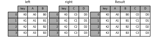
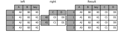
It is worth spending some time understanding the result of the many-to-many join case. In SQL / standard relational algebra, if a key combination appears more than once in both tables, the resulting table will have the Cartesian product of the associated data. Here is a very basic example with one unique key combination:
In [39]: left = pd.DataFrame({'key': ['K0', 'K1', 'K2', 'K3'],....: 'A': ['A0', 'A1', 'A2', 'A3'],....: 'B': ['B0', 'B1', 'B2', 'B3']})....:In [40]: right = pd.DataFrame({'key': ['K0', 'K1', 'K2', 'K3'],....: 'C': ['C0', 'C1', 'C2', 'C3'],....: 'D': ['D0', 'D1', 'D2', 'D3']})....:In [41]: result = pd.merge(left, right, on='key')
Here is a more complicated example with multiple join keys. Only the keys
appearing in left and right are present (the intersection), since
how='inner' by default.
In [42]: left = pd.DataFrame({'key1': ['K0', 'K0', 'K1', 'K2'],....: 'key2': ['K0', 'K1', 'K0', 'K1'],....: 'A': ['A0', 'A1', 'A2', 'A3'],....: 'B': ['B0', 'B1', 'B2', 'B3']})....:In [43]: right = pd.DataFrame({'key1': ['K0', 'K1', 'K1', 'K2'],....: 'key2': ['K0', 'K0', 'K0', 'K0'],....: 'C': ['C0', 'C1', 'C2', 'C3'],....: 'D': ['D0', 'D1', 'D2', 'D3']})....:In [44]: result = pd.merge(left, right, on=['key1', 'key2'])

The how argument to merge specifies how to determine which keys are to
be included in the resulting table. If a key combination does not appear in
either the left or right tables, the values in the joined table will be
NA. Here is a summary of the how options and their SQL equivalent names:
| Merge method | SQL Join Name | Description |
|---|---|---|
| left | LEFT OUTER JOIN | Use keys from left frame only |
| right | RIGHT OUTER JOIN | Use keys from right frame only |
| outer | FULL OUTER JOIN | Use union of keys from both frames |
| inner | INNER JOIN | Use intersection of keys from both frames |
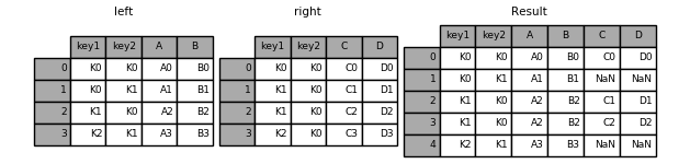
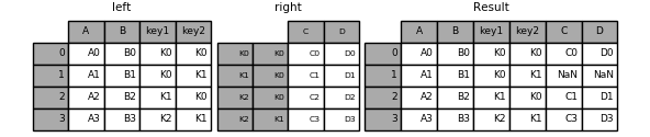
In [45]: result = pd.merge(left, right, how='left', on=['key1', 'key2'])
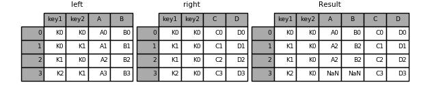
In [46]: result = pd.merge(left, right, how='right', on=['key1', 'key2'])
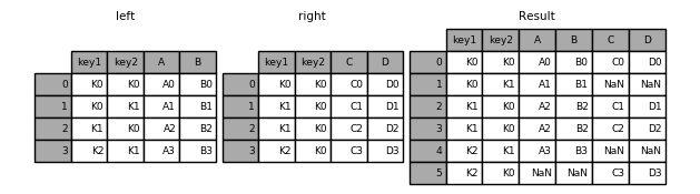
In [47]: result = pd.merge(left, right, how='outer', on=['key1', 'key2'])
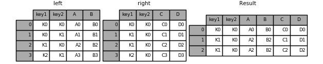
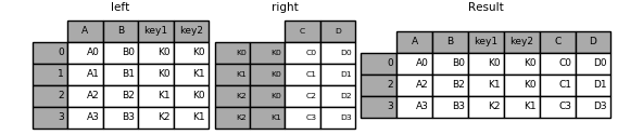
In [48]: result = pd.merge(left, right, how='inner', on=['key1', 'key2'])
Here is another example with duplicate join keys in DataFrames:
In [49]: left = pd.DataFrame({'A': [1, 2], 'B': [2, 2]})In [50]: right = pd.DataFrame({'A': [4, 5, 6], 'B': [2, 2, 2]})In [51]: result = pd.merge(left, right, on='B', how='outer')
::: danger Warning
Joining / merging on duplicate keys can cause a returned frame that is the multiplication of the row dimensions, which may result in memory overflow. It is the user’ s responsibility to manage duplicate values in keys before joining large DataFrames.
:::
Checking for duplicate keys
New in version 0.21.0.
Users can use the validate argument to automatically check whether there
are unexpected duplicates in their merge keys. Key uniqueness is checked before
merge operations and so should protect against memory overflows. Checking key
uniqueness is also a good way to ensure user data structures are as expected.
In the following example, there are duplicate values of B in the right
DataFrame. As this is not a one-to-one merge – as specified in the
validate argument – an exception will be raised.
In [52]: left = pd.DataFrame({'A' : [1,2], 'B' : [1, 2]})In [53]: right = pd.DataFrame({'A' : [4,5,6], 'B': [2, 2, 2]})
In [53]: result = pd.merge(left, right, on='B', how='outer', validate="one_to_one")...MergeError: Merge keys are not unique in right dataset; not a one-to-one merge
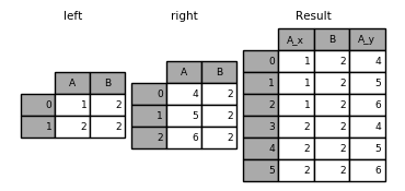
If the user is aware of the duplicates in the right DataFrame but wants to
ensure there are no duplicates in the left DataFrame, one can use the
validate='one_to_many' argument instead, which will not raise an exception.
In [54]: pd.merge(left, right, on='B', how='outer', validate="one_to_many")Out[54]:A_x B A_y0 1 1 NaN1 2 2 4.02 2 2 5.03 2 2 6.0
The merge indicator
merge() accepts the argument indicator. If True, a
Categorical-type column called _merge will be added to the output object
that takes on values:
| Observation Origin | _merge value |
|---|---|
| Merge key only in ‘left’ frame | left_only |
| Merge key only in ‘right’ frame | right_only |
| Merge key in both frames | both |
In [55]: df1 = pd.DataFrame({'col1': [0, 1], 'col_left': ['a', 'b']})In [56]: df2 = pd.DataFrame({'col1': [1, 2, 2], 'col_right': [2, 2, 2]})In [57]: pd.merge(df1, df2, on='col1', how='outer', indicator=True)Out[57]:col1 col_left col_right _merge0 0 a NaN left_only1 1 b 2.0 both2 2 NaN 2.0 right_only3 2 NaN 2.0 right_only
The indicator argument will also accept string arguments, in which case the indicator function will use the value of the passed string as the name for the indicator column.
In [58]: pd.merge(df1, df2, on='col1', how='outer', indicator='indicator_column')Out[58]:col1 col_left col_right indicator_column0 0 a NaN left_only1 1 b 2.0 both2 2 NaN 2.0 right_only3 2 NaN 2.0 right_only
Merge dtypes
New in version 0.19.0.
Merging will preserve the dtype of the join keys.
In [59]: left = pd.DataFrame({'key': [1], 'v1': [10]})In [60]: leftOut[60]:key v10 1 10In [61]: right = pd.DataFrame({'key': [1, 2], 'v1': [20, 30]})In [62]: rightOut[62]:key v10 1 201 2 30
We are able to preserve the join keys:
In [63]: pd.merge(left, right, how='outer')Out[63]:key v10 1 101 1 202 2 30In [64]: pd.merge(left, right, how='outer').dtypesOut[64]:key int64v1 int64dtype: object
Of course if you have missing values that are introduced, then the resulting dtype will be upcast.
In [65]: pd.merge(left, right, how='outer', on='key')Out[65]:key v1_x v1_y0 1 10.0 201 2 NaN 30In [66]: pd.merge(left, right, how='outer', on='key').dtypesOut[66]:key int64v1_x float64v1_y int64dtype: object
New in version 0.20.0.
Merging will preserve category dtypes of the mergands. See also the section on categoricals.
The left frame.
In [67]: from pandas.api.types import CategoricalDtypeIn [68]: X = pd.Series(np.random.choice(['foo', 'bar'], size=(10,)))In [69]: X = X.astype(CategoricalDtype(categories=['foo', 'bar']))In [70]: left = pd.DataFrame({'X': X,....: 'Y': np.random.choice(['one', 'two', 'three'],....: size=(10,))})....:In [71]: leftOut[71]:X Y0 bar one1 foo one2 foo three3 bar three4 foo one5 bar one6 bar three7 bar three8 bar three9 foo threeIn [72]: left.dtypesOut[72]:X categoryY objectdtype: object
The right frame.
In [73]: right = pd.DataFrame({'X': pd.Series(['foo', 'bar'],....: dtype=CategoricalDtype(['foo', 'bar'])),....: 'Z': [1, 2]})....:In [74]: rightOut[74]:X Z0 foo 11 bar 2In [75]: right.dtypesOut[75]:X categoryZ int64dtype: object
The merged result:
In [76]: result = pd.merge(left, right, how='outer')In [77]: resultOut[77]:X Y Z0 bar one 21 bar three 22 bar one 23 bar three 24 bar three 25 bar three 26 foo one 17 foo three 18 foo one 19 foo three 1In [78]: result.dtypesOut[78]:X categoryY objectZ int64dtype: object
::: tip Note
The category dtypes must be exactly the same, meaning the same categories and the ordered attribute.
Otherwise the result will coerce to object dtype.
:::
::: tip Note
Merging on category dtypes that are the same can be quite performant compared to object dtype merging.
:::
Joining on index
DataFrame.join() is a convenient method for combining the columns of two
potentially differently-indexed DataFrames into a single result
DataFrame. Here is a very basic example:
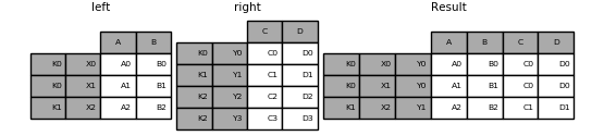
In [79]: left = pd.DataFrame({'A': ['A0', 'A1', 'A2'],....: 'B': ['B0', 'B1', 'B2']},....: index=['K0', 'K1', 'K2'])....:In [80]: right = pd.DataFrame({'C': ['C0', 'C2', 'C3'],....: 'D': ['D0', 'D2', 'D3']},....: index=['K0', 'K2', 'K3'])....:In [81]: result = left.join(right)
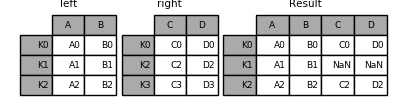
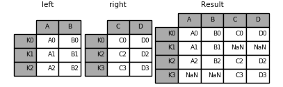
In [82]: result = left.join(right, how='outer')
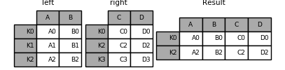
The same as above, but with how='inner'.
In [83]: result = left.join(right, how='inner')
The data alignment here is on the indexes (row labels). This same behavior can
be achieved using merge plus additional arguments instructing it to use the
indexes:
In [84]: result = pd.merge(left, right, left_index=True, right_index=True, how='outer')

In [85]: result = pd.merge(left, right, left_index=True, right_index=True, how='inner');

Joining key columns on an index
join() takes an optional on argument which may be a column
or multiple column names, which specifies that the passed DataFrame is to be
aligned on that column in the DataFrame. These two function calls are
completely equivalent:
left.join(right, on=key_or_keys)pd.merge(left, right, left_on=key_or_keys, right_index=True,how='left', sort=False)
Obviously you can choose whichever form you find more convenient. For
many-to-one joins (where one of the DataFrame’s is already indexed by the
join key), using join may be more convenient. Here is a simple example:
In [86]: left = pd.DataFrame({'A': ['A0', 'A1', 'A2', 'A3'],....: 'B': ['B0', 'B1', 'B2', 'B3'],....: 'key': ['K0', 'K1', 'K0', 'K1']})....:In [87]: right = pd.DataFrame({'C': ['C0', 'C1'],....: 'D': ['D0', 'D1']},....: index=['K0', 'K1'])....:In [88]: result = left.join(right, on='key')
In [89]: result = pd.merge(left, right, left_on='key', right_index=True,....: how='left', sort=False);....:

To join on multiple keys, the passed DataFrame must have a MultiIndex:
In [90]: left = pd.DataFrame({'A': ['A0', 'A1', 'A2', 'A3'],....: 'B': ['B0', 'B1', 'B2', 'B3'],....: 'key1': ['K0', 'K0', 'K1', 'K2'],....: 'key2': ['K0', 'K1', 'K0', 'K1']})....:In [91]: index = pd.MultiIndex.from_tuples([('K0', 'K0'), ('K1', 'K0'),....: ('K2', 'K0'), ('K2', 'K1')])....:In [92]: right = pd.DataFrame({'C': ['C0', 'C1', 'C2', 'C3'],....: 'D': ['D0', 'D1', 'D2', 'D3']},....: index=index)....:
Now this can be joined by passing the two key column names:
In [93]: result = left.join(right, on=['key1', 'key2'])
The default for DataFrame.join is to perform a left join (essentially a
“VLOOKUP” operation, for Excel users), which uses only the keys found in the
calling DataFrame. Other join types, for example inner join, can be just as
easily performed:
In [94]: result = left.join(right, on=['key1', 'key2'], how='inner')
As you can see, this drops any rows where there was no match.
Joining a single Index to a MultiIndex
You can join a singly-indexed DataFrame with a level of a MultiIndexed DataFrame.
The level will match on the name of the index of the singly-indexed frame against
a level name of the MultiIndexed frame.
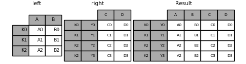
In [95]: left = pd.DataFrame({'A': ['A0', 'A1', 'A2'],....: 'B': ['B0', 'B1', 'B2']},....: index=pd.Index(['K0', 'K1', 'K2'], name='key'))....:In [96]: index = pd.MultiIndex.from_tuples([('K0', 'Y0'), ('K1', 'Y1'),....: ('K2', 'Y2'), ('K2', 'Y3')],....: names=['key', 'Y'])....:In [97]: right = pd.DataFrame({'C': ['C0', 'C1', 'C2', 'C3'],....: 'D': ['D0', 'D1', 'D2', 'D3']},....: index=index)....:In [98]: result = left.join(right, how='inner')

This is equivalent but less verbose and more memory efficient / faster than this.
In [99]: result = pd.merge(left.reset_index(), right.reset_index(),....: on=['key'], how='inner').set_index(['key','Y'])....:
Joining with two MultiIndexes
This is supported in a limited way, provided that the index for the right argument is completely used in the join, and is a subset of the indices in the left argument, as in this example:
In [100]: leftindex = pd.MultiIndex.from_product([list('abc'), list('xy'), [1, 2]],.....: names=['abc', 'xy', 'num']).....:In [101]: left = pd.DataFrame({'v1': range(12)}, index=leftindex)In [102]: leftOut[102]:v1abc xy numa x 1 02 1y 1 22 3b x 1 42 5y 1 62 7c x 1 82 9y 1 102 11In [103]: rightindex = pd.MultiIndex.from_product([list('abc'), list('xy')],.....: names=['abc', 'xy']).....:In [104]: right = pd.DataFrame({'v2': [100 * i for i in range(1, 7)]}, index=rightindex)In [105]: rightOut[105]:v2abc xya x 100y 200b x 300y 400c x 500y 600In [106]: left.join(right, on=['abc', 'xy'], how='inner')Out[106]:v1 v2abc xy numa x 1 0 1002 1 100y 1 2 2002 3 200b x 1 4 3002 5 300y 1 6 4002 7 400c x 1 8 5002 9 500y 1 10 6002 11 600
If that condition is not satisfied, a join with two multi-indexes can be done using the following code.
In [107]: leftindex = pd.MultiIndex.from_tuples([('K0', 'X0'), ('K0', 'X1'),.....: ('K1', 'X2')],.....: names=['key', 'X']).....:In [108]: left = pd.DataFrame({'A': ['A0', 'A1', 'A2'],.....: 'B': ['B0', 'B1', 'B2']},.....: index=leftindex).....:In [109]: rightindex = pd.MultiIndex.from_tuples([('K0', 'Y0'), ('K1', 'Y1'),.....: ('K2', 'Y2'), ('K2', 'Y3')],.....: names=['key', 'Y']).....:In [110]: right = pd.DataFrame({'C': ['C0', 'C1', 'C2', 'C3'],.....: 'D': ['D0', 'D1', 'D2', 'D3']},.....: index=rightindex).....:In [111]: result = pd.merge(left.reset_index(), right.reset_index(),.....: on=['key'], how='inner').set_index(['key', 'X', 'Y']).....:
Merging on a combination of columns and index levels
New in version 0.23.
Strings passed as the on, left_on, and right_on parameters
may refer to either column names or index level names. This enables merging
DataFrame instances on a combination of index levels and columns without
resetting indexes.
In [112]: left_index = pd.Index(['K0', 'K0', 'K1', 'K2'], name='key1')In [113]: left = pd.DataFrame({'A': ['A0', 'A1', 'A2', 'A3'],.....: 'B': ['B0', 'B1', 'B2', 'B3'],.....: 'key2': ['K0', 'K1', 'K0', 'K1']},.....: index=left_index).....:In [114]: right_index = pd.Index(['K0', 'K1', 'K2', 'K2'], name='key1')In [115]: right = pd.DataFrame({'C': ['C0', 'C1', 'C2', 'C3'],.....: 'D': ['D0', 'D1', 'D2', 'D3'],.....: 'key2': ['K0', 'K0', 'K0', 'K1']},.....: index=right_index).....:In [116]: result = left.merge(right, on=['key1', 'key2'])

::: tip Note
When DataFrames are merged on a string that matches an index level in both frames, the index level is preserved as an index level in the resulting DataFrame.
:::
::: tip Note
When DataFrames are merged using only some of the levels of a MultiIndex,
the extra levels will be dropped from the resulting merge. In order to
preserve those levels, use reset_index on those level names to move
those levels to columns prior to doing the merge.
:::
::: tip Note
If a string matches both a column name and an index level name, then a warning is issued and the column takes precedence. This will result in an ambiguity error in a future version.
:::
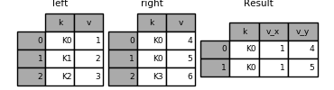
Overlapping value columns
The merge suffixes argument takes a tuple of list of strings to append to
overlapping column names in the input DataFrames to disambiguate the result
columns:
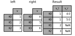
In [117]: left = pd.DataFrame({'k': ['K0', 'K1', 'K2'], 'v': [1, 2, 3]})In [118]: right = pd.DataFrame({'k': ['K0', 'K0', 'K3'], 'v': [4, 5, 6]})In [119]: result = pd.merge(left, right, on='k')
In [120]: result = pd.merge(left, right, on='k', suffixes=['_l', '_r'])

DataFrame.join() has lsuffix and rsuffix arguments which behave
similarly.
In [121]: left = left.set_index('k')In [122]: right = right.set_index('k')In [123]: result = left.join(right, lsuffix='_l', rsuffix='_r')
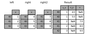
Joining multiple DataFrames
A list or tuple of DataFrames can also be passed to join()
to join them together on their indexes.
In [124]: right2 = pd.DataFrame({'v': [7, 8, 9]}, index=['K1', 'K1', 'K2'])In [125]: result = left.join([right, right2])
Merging together values within Series or DataFrame columns
Another fairly common situation is to have two like-indexed (or similarly
indexed) Series or DataFrame objects and wanting to “patch” values in
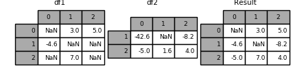
one object from values for matching indices in the other. Here is an example:
In [126]: df1 = pd.DataFrame([[np.nan, 3., 5.], [-4.6, np.nan, np.nan],.....: [np.nan, 7., np.nan]]).....:In [127]: df2 = pd.DataFrame([[-42.6, np.nan, -8.2], [-5., 1.6, 4]],.....: index=[1, 2]).....:
For this, use the combine_first() method:
In [128]: result = df1.combine_first(df2)
Note that this method only takes values from the right DataFrame if they are
missing in the left DataFrame. A related method, update(),
alters non-NA values in place:
In [129]: df1.update(df2)

Timeseries friendly merging
Merging ordered data
A merge_ordered() function allows combining time series and other
ordered data. In particular it has an optional fill_method keyword to
fill/interpolate missing data:
In [130]: left = pd.DataFrame({'k': ['K0', 'K1', 'K1', 'K2'],.....: 'lv': [1, 2, 3, 4],.....: 's': ['a', 'b', 'c', 'd']}).....:In [131]: right = pd.DataFrame({'k': ['K1', 'K2', 'K4'],.....: 'rv': [1, 2, 3]}).....:In [132]: pd.merge_ordered(left, right, fill_method='ffill', left_by='s')Out[132]:k lv s rv0 K0 1.0 a NaN1 K1 1.0 a 1.02 K2 1.0 a 2.03 K4 1.0 a 3.04 K1 2.0 b 1.05 K2 2.0 b 2.06 K4 2.0 b 3.07 K1 3.0 c 1.08 K2 3.0 c 2.09 K4 3.0 c 3.010 K1 NaN d 1.011 K2 4.0 d 2.012 K4 4.0 d 3.0
Merging asof
New in version 0.19.0.
A merge_asof() is similar to an ordered left-join except that we match on
nearest key rather than equal keys. For each row in the left DataFrame,
we select the last row in the right DataFrame whose on key is less
than the left’s key. Both DataFrames must be sorted by the key.
Optionally an asof merge can perform a group-wise merge. This matches the
by key equally, in addition to the nearest match on the on key.
For example; we might have trades and quotes and we want to asof
merge them.
In [133]: trades = pd.DataFrame({.....: 'time': pd.to_datetime(['20160525 13:30:00.023',.....: '20160525 13:30:00.038',.....: '20160525 13:30:00.048',.....: '20160525 13:30:00.048',.....: '20160525 13:30:00.048']),.....: 'ticker': ['MSFT', 'MSFT',.....: 'GOOG', 'GOOG', 'AAPL'],.....: 'price': [51.95, 51.95,.....: 720.77, 720.92, 98.00],.....: 'quantity': [75, 155,.....: 100, 100, 100]},.....: columns=['time', 'ticker', 'price', 'quantity']).....:In [134]: quotes = pd.DataFrame({.....: 'time': pd.to_datetime(['20160525 13:30:00.023',.....: '20160525 13:30:00.023',.....: '20160525 13:30:00.030',.....: '20160525 13:30:00.041',.....: '20160525 13:30:00.048',.....: '20160525 13:30:00.049',.....: '20160525 13:30:00.072',.....: '20160525 13:30:00.075']),.....: 'ticker': ['GOOG', 'MSFT', 'MSFT',.....: 'MSFT', 'GOOG', 'AAPL', 'GOOG',.....: 'MSFT'],.....: 'bid': [720.50, 51.95, 51.97, 51.99,.....: 720.50, 97.99, 720.50, 52.01],.....: 'ask': [720.93, 51.96, 51.98, 52.00,.....: 720.93, 98.01, 720.88, 52.03]},.....: columns=['time', 'ticker', 'bid', 'ask']).....:
In [135]: tradesOut[135]:time ticker price quantity0 2016-05-25 13:30:00.023 MSFT 51.95 751 2016-05-25 13:30:00.038 MSFT 51.95 1552 2016-05-25 13:30:00.048 GOOG 720.77 1003 2016-05-25 13:30:00.048 GOOG 720.92 1004 2016-05-25 13:30:00.048 AAPL 98.00 100In [136]: quotesOut[136]:time ticker bid ask0 2016-05-25 13:30:00.023 GOOG 720.50 720.931 2016-05-25 13:30:00.023 MSFT 51.95 51.962 2016-05-25 13:30:00.030 MSFT 51.97 51.983 2016-05-25 13:30:00.041 MSFT 51.99 52.004 2016-05-25 13:30:00.048 GOOG 720.50 720.935 2016-05-25 13:30:00.049 AAPL 97.99 98.016 2016-05-25 13:30:00.072 GOOG 720.50 720.887 2016-05-25 13:30:00.075 MSFT 52.01 52.03
By default we are taking the asof of the quotes.
In [137]: pd.merge_asof(trades, quotes,.....: on='time',.....: by='ticker').....:Out[137]:time ticker price quantity bid ask0 2016-05-25 13:30:00.023 MSFT 51.95 75 51.95 51.961 2016-05-25 13:30:00.038 MSFT 51.95 155 51.97 51.982 2016-05-25 13:30:00.048 GOOG 720.77 100 720.50 720.933 2016-05-25 13:30:00.048 GOOG 720.92 100 720.50 720.934 2016-05-25 13:30:00.048 AAPL 98.00 100 NaN NaN
We only asof within 2ms between the quote time and the trade time.
In [138]: pd.merge_asof(trades, quotes,.....: on='time',.....: by='ticker',.....: tolerance=pd.Timedelta('2ms')).....:Out[138]:time ticker price quantity bid ask0 2016-05-25 13:30:00.023 MSFT 51.95 75 51.95 51.961 2016-05-25 13:30:00.038 MSFT 51.95 155 NaN NaN2 2016-05-25 13:30:00.048 GOOG 720.77 100 720.50 720.933 2016-05-25 13:30:00.048 GOOG 720.92 100 720.50 720.934 2016-05-25 13:30:00.048 AAPL 98.00 100 NaN NaN
We only asof within 10ms between the quote time and the trade time and we
exclude exact matches on time. Note that though we exclude the exact matches
(of the quotes), prior quotes do propagate to that point in time.
In [139]: pd.merge_asof(trades, quotes,.....: on='time',.....: by='ticker',.....: tolerance=pd.Timedelta('10ms'),.....: allow_exact_matches=False).....:Out[139]:time ticker price quantity bid ask0 2016-05-25 13:30:00.023 MSFT 51.95 75 NaN NaN1 2016-05-25 13:30:00.038 MSFT 51.95 155 51.97 51.982 2016-05-25 13:30:00.048 GOOG 720.77 100 NaN NaN3 2016-05-25 13:30:00.048 GOOG 720.92 100 NaN NaN4 2016-05-25 13:30:00.048 AAPL 98.00 100 NaN NaN

若有收获,就点个赞吧
0 人点赞
