Reshaping and pivot tables
Reshaping by pivoting DataFrame objects
Data is often stored in so-called “stacked” or “record” format:
In [1]: dfOut[1]:date variable value0 2000-01-03 A 0.4691121 2000-01-04 A -0.2828632 2000-01-05 A -1.5090593 2000-01-03 B -1.1356324 2000-01-04 B 1.2121125 2000-01-05 B -0.1732156 2000-01-03 C 0.1192097 2000-01-04 C -1.0442368 2000-01-05 C -0.8618499 2000-01-03 D -2.10456910 2000-01-04 D -0.49492911 2000-01-05 D 1.071804
For the curious here is how the above DataFrame was created:
import pandas.util.testing as tmtm.N = 3def unpivot(frame):N, K = frame.shapedata = {'value': frame.to_numpy().ravel('F'),'variable': np.asarray(frame.columns).repeat(N),'date': np.tile(np.asarray(frame.index), K)}return pd.DataFrame(data, columns=['date', 'variable', 'value'])df = unpivot(tm.makeTimeDataFrame())
To select out everything for variable A we could do:
In [2]: df[df['variable'] == 'A']Out[2]:date variable value0 2000-01-03 A 0.4691121 2000-01-04 A -0.2828632 2000-01-05 A -1.509059
But suppose we wish to do time series operations with the variables. A better
representation would be where the columns are the unique variables and an
index of dates identifies individual observations. To reshape the data into
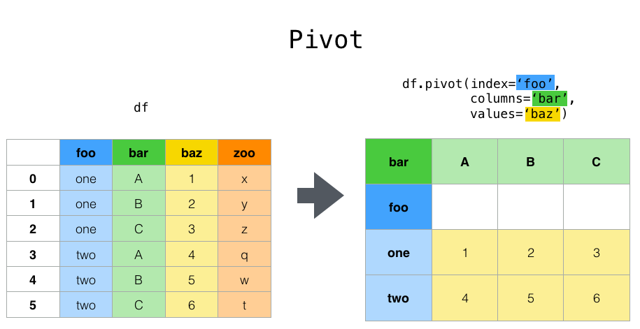
this form, we use the DataFrame.pivot() method (also implemented as a
top level function pivot()):
In [3]: df.pivot(index='date', columns='variable', values='value')Out[3]:variable A B C Ddate2000-01-03 0.469112 -1.135632 0.119209 -2.1045692000-01-04 -0.282863 1.212112 -1.044236 -0.4949292000-01-05 -1.509059 -0.173215 -0.861849 1.071804
If the values argument is omitted, and the input DataFrame has more than
one column of values which are not used as column or index inputs to pivot,
then the resulting “pivoted” DataFrame will have hierarchical columns whose topmost level indicates the respective value
column:
In [4]: df['value2'] = df['value'] * 2In [5]: pivoted = df.pivot(index='date', columns='variable')In [6]: pivotedOut[6]:value value2variable A B C D A B C Ddate2000-01-03 0.469112 -1.135632 0.119209 -2.104569 0.938225 -2.271265 0.238417 -4.2091382000-01-04 -0.282863 1.212112 -1.044236 -0.494929 -0.565727 2.424224 -2.088472 -0.9898592000-01-05 -1.509059 -0.173215 -0.861849 1.071804 -3.018117 -0.346429 -1.723698 2.143608
You can then select subsets from the pivoted DataFrame:
In [7]: pivoted['value2']Out[7]:variable A B C Ddate2000-01-03 0.938225 -2.271265 0.238417 -4.2091382000-01-04 -0.565727 2.424224 -2.088472 -0.9898592000-01-05 -3.018117 -0.346429 -1.723698 2.143608
Note that this returns a view on the underlying data in the case where the data are homogeneously-typed.
::: tip Note
pivot() will error with a ValueError: Index contains duplicate
entries, cannot reshape if the index/column pair is not unique. In this
case, consider using pivot_table() which is a generalization
of pivot that can handle duplicate values for one index/column pair.
:::
Reshaping by stacking and unstacking
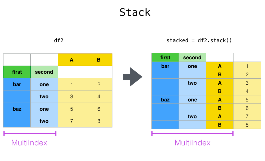
Closely related to the pivot() method are the related
stack() and unstack() methods available on
Series and DataFrame. These methods are designed to work together with
MultiIndex objects (see the section on hierarchical indexing). Here are essentially what these methods do:
stack: “pivot” a level of the (possibly hierarchical) column labels, returning aDataFramewith an index with a new inner-most level of row labels.unstack: (inverse operation ofstack) “pivot” a level of the (possibly hierarchical) row index to the column axis, producing a reshapedDataFramewith a new inner-most level of column labels.
The clearest way to explain is by example. Let’s take a prior example data set from the hierarchical indexing section:
In [8]: tuples = list(zip(*[['bar', 'bar', 'baz', 'baz',...: 'foo', 'foo', 'qux', 'qux'],...: ['one', 'two', 'one', 'two',...: 'one', 'two', 'one', 'two']]))...:In [9]: index = pd.MultiIndex.from_tuples(tuples, names=['first', 'second'])In [10]: df = pd.DataFrame(np.random.randn(8, 2), index=index, columns=['A', 'B'])In [11]: df2 = df[:4]In [12]: df2Out[12]:A Bfirst secondbar one 0.721555 -0.706771two -1.039575 0.271860baz one -0.424972 0.567020two 0.276232 -1.087401
The stack function “compresses” a level in the DataFrame’s columns to
produce either:
- A
Series, in the case of a simple column Index. - A
DataFrame, in the case of aMultiIndexin the columns.
If the columns have a MultiIndex, you can choose which level to stack. The
stacked level becomes the new lowest level in a MultiIndex on the columns:
In [13]: stacked = df2.stack()In [14]: stackedOut[14]:first secondbar one A 0.721555B -0.706771two A -1.039575B 0.271860baz one A -0.424972B 0.567020two A 0.276232B -1.087401dtype: float64
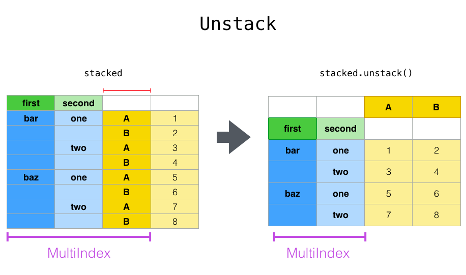
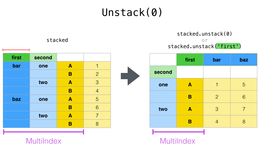
With a “stacked” DataFrame or Series (having a MultiIndex as the
index), the inverse operation of stack is unstack, which by default
unstacks the last level:
In [15]: stacked.unstack()Out[15]:A Bfirst secondbar one 0.721555 -0.706771two -1.039575 0.271860baz one -0.424972 0.567020two 0.276232 -1.087401In [16]: stacked.unstack(1)Out[16]:second one twofirstbar A 0.721555 -1.039575B -0.706771 0.271860baz A -0.424972 0.276232B 0.567020 -1.087401In [17]: stacked.unstack(0)Out[17]:first bar bazsecondone A 0.721555 -0.424972B -0.706771 0.567020two A -1.039575 0.276232B 0.271860 -1.087401
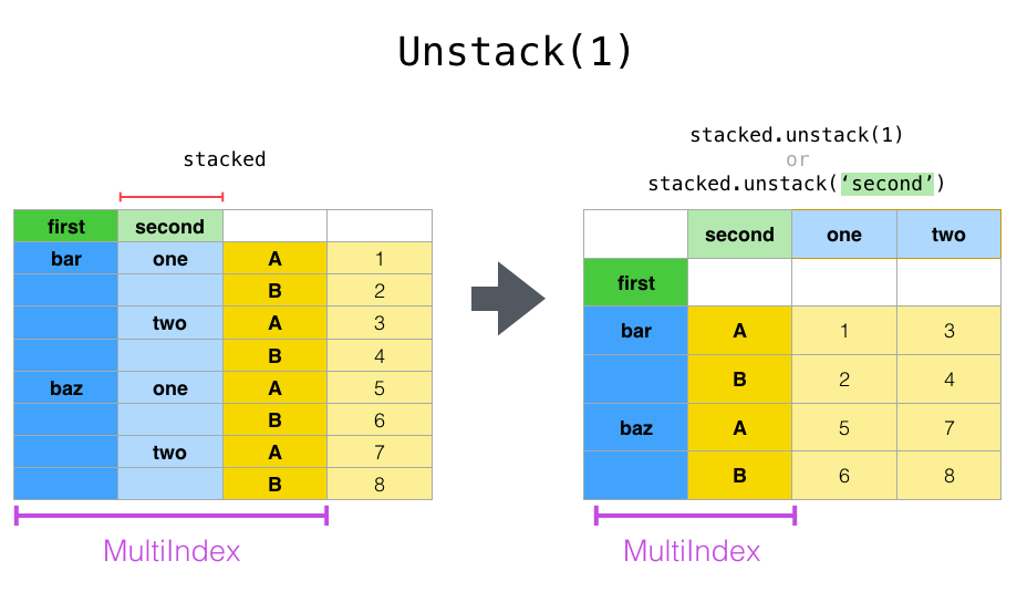
If the indexes have names, you can use the level names instead of specifying the level numbers:
In [18]: stacked.unstack('second')Out[18]:second one twofirstbar A 0.721555 -1.039575B -0.706771 0.271860baz A -0.424972 0.276232B 0.567020 -1.087401
Notice that the stack and unstack methods implicitly sort the index
levels involved. Hence a call to stack and then unstack, or vice versa,
will result in a sorted copy of the original DataFrame or Series:
In [19]: index = pd.MultiIndex.from_product([[2, 1], ['a', 'b']])In [20]: df = pd.DataFrame(np.random.randn(4), index=index, columns=['A'])In [21]: dfOut[21]:A2 a -0.370647b -1.1578921 a -1.344312b 0.844885In [22]: all(df.unstack().stack() == df.sort_index())Out[22]: True
The above code will raise a TypeError if the call to sort_index is
removed.
Multiple levels
You may also stack or unstack more than one level at a time by passing a list of levels, in which case the end result is as if each level in the list were processed individually.
In [23]: columns = pd.MultiIndex.from_tuples([....: ('A', 'cat', 'long'), ('B', 'cat', 'long'),....: ('A', 'dog', 'short'), ('B', 'dog', 'short')],....: names=['exp', 'animal', 'hair_length']....: )....:In [24]: df = pd.DataFrame(np.random.randn(4, 4), columns=columns)In [25]: dfOut[25]:exp A B A Banimal cat cat dog doghair_length long long short short0 1.075770 -0.109050 1.643563 -1.4693881 0.357021 -0.674600 -1.776904 -0.9689142 -1.294524 0.413738 0.276662 -0.4720353 -0.013960 -0.362543 -0.006154 -0.923061In [26]: df.stack(level=['animal', 'hair_length'])Out[26]:exp A Banimal hair_length0 cat long 1.075770 -0.109050dog short 1.643563 -1.4693881 cat long 0.357021 -0.674600dog short -1.776904 -0.9689142 cat long -1.294524 0.413738dog short 0.276662 -0.4720353 cat long -0.013960 -0.362543dog short -0.006154 -0.923061
The list of levels can contain either level names or level numbers (but not a mixture of the two).
# df.stack(level=['animal', 'hair_length'])# from above is equivalent to:In [27]: df.stack(level=[1, 2])Out[27]:exp A Banimal hair_length0 cat long 1.075770 -0.109050dog short 1.643563 -1.4693881 cat long 0.357021 -0.674600dog short -1.776904 -0.9689142 cat long -1.294524 0.413738dog short 0.276662 -0.4720353 cat long -0.013960 -0.362543dog short -0.006154 -0.923061
Missing data
These functions are intelligent about handling missing data and do not expect
each subgroup within the hierarchical index to have the same set of labels.
They also can handle the index being unsorted (but you can make it sorted by
calling sort_index, of course). Here is a more complex example:
In [28]: columns = pd.MultiIndex.from_tuples([('A', 'cat'), ('B', 'dog'),....: ('B', 'cat'), ('A', 'dog')],....: names=['exp', 'animal'])....:In [29]: index = pd.MultiIndex.from_product([('bar', 'baz', 'foo', 'qux'),....: ('one', 'two')],....: names=['first', 'second'])....:In [30]: df = pd.DataFrame(np.random.randn(8, 4), index=index, columns=columns)In [31]: df2 = df.iloc[[0, 1, 2, 4, 5, 7]]In [32]: df2Out[32]:exp A B Aanimal cat dog cat dogfirst secondbar one 0.895717 0.805244 -1.206412 2.565646two 1.431256 1.340309 -1.170299 -0.226169baz one 0.410835 0.813850 0.132003 -0.827317foo one -1.413681 1.607920 1.024180 0.569605two 0.875906 -2.211372 0.974466 -2.006747qux two -1.226825 0.769804 -1.281247 -0.727707
As mentioned above, stack can be called with a level argument to select
which level in the columns to stack:
In [33]: df2.stack('exp')Out[33]:animal cat dogfirst second expbar one A 0.895717 2.565646B -1.206412 0.805244two A 1.431256 -0.226169B -1.170299 1.340309baz one A 0.410835 -0.827317B 0.132003 0.813850foo one A -1.413681 0.569605B 1.024180 1.607920two A 0.875906 -2.006747B 0.974466 -2.211372qux two A -1.226825 -0.727707B -1.281247 0.769804In [34]: df2.stack('animal')Out[34]:exp A Bfirst second animalbar one cat 0.895717 -1.206412dog 2.565646 0.805244two cat 1.431256 -1.170299dog -0.226169 1.340309baz one cat 0.410835 0.132003dog -0.827317 0.813850foo one cat -1.413681 1.024180dog 0.569605 1.607920two cat 0.875906 0.974466dog -2.006747 -2.211372qux two cat -1.226825 -1.281247dog -0.727707 0.769804
Unstacking can result in missing values if subgroups do not have the same
set of labels. By default, missing values will be replaced with the default
fill value for that data type, NaN for float, NaT for datetimelike,
etc. For integer types, by default data will converted to float and missing
values will be set to NaN.
In [35]: df3 = df.iloc[[0, 1, 4, 7], [1, 2]]In [36]: df3Out[36]:exp Banimal dog catfirst secondbar one 0.805244 -1.206412two 1.340309 -1.170299foo one 1.607920 1.024180qux two 0.769804 -1.281247In [37]: df3.unstack()Out[37]:exp Banimal dog catsecond one two one twofirstbar 0.805244 1.340309 -1.206412 -1.170299foo 1.607920 NaN 1.024180 NaNqux NaN 0.769804 NaN -1.281247
New in version 0.18.0.
Alternatively, unstack takes an optional fill_value argument, for specifying
the value of missing data.
In [38]: df3.unstack(fill_value=-1e9)Out[38]:exp Banimal dog catsecond one two one twofirstbar 8.052440e-01 1.340309e+00 -1.206412e+00 -1.170299e+00foo 1.607920e+00 -1.000000e+09 1.024180e+00 -1.000000e+09qux -1.000000e+09 7.698036e-01 -1.000000e+09 -1.281247e+00
With a MultiIndex
Unstacking when the columns are a MultiIndex is also careful about doing
the right thing:
In [39]: df[:3].unstack(0)Out[39]:exp A B Aanimal cat dog cat dogfirst bar baz bar baz bar baz bar bazsecondone 0.895717 0.410835 0.805244 0.81385 -1.206412 0.132003 2.565646 -0.827317two 1.431256 NaN 1.340309 NaN -1.170299 NaN -0.226169 NaNIn [40]: df2.unstack(1)Out[40]:exp A B Aanimal cat dog cat dogsecond one two one two one two one twofirstbar 0.895717 1.431256 0.805244 1.340309 -1.206412 -1.170299 2.565646 -0.226169baz 0.410835 NaN 0.813850 NaN 0.132003 NaN -0.827317 NaNfoo -1.413681 0.875906 1.607920 -2.211372 1.024180 0.974466 0.569605 -2.006747qux NaN -1.226825 NaN 0.769804 NaN -1.281247 NaN -0.727707
Reshaping by Melt
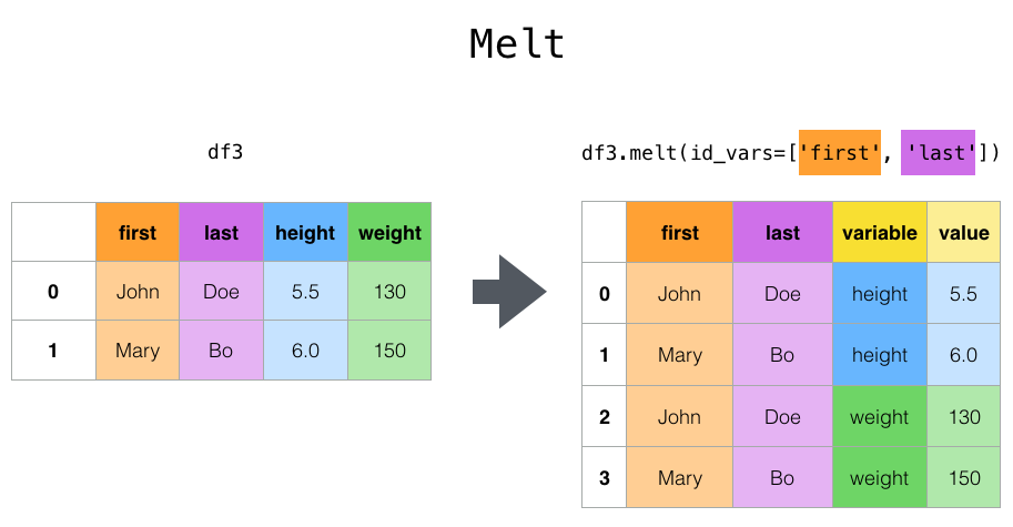
The top-level melt() function and the corresponding DataFrame.melt()
are useful to massage a DataFrame into a format where one or more columns
are identifier variables, while all other columns, considered measured
variables, are “unpivoted” to the row axis, leaving just two non-identifier
columns, “variable” and “value”. The names of those columns can be customized
by supplying the var_name and value_name parameters.
For instance,
In [41]: cheese = pd.DataFrame({'first': ['John', 'Mary'],....: 'last': ['Doe', 'Bo'],....: 'height': [5.5, 6.0],....: 'weight': [130, 150]})....:In [42]: cheeseOut[42]:first last height weight0 John Doe 5.5 1301 Mary Bo 6.0 150In [43]: cheese.melt(id_vars=['first', 'last'])Out[43]:first last variable value0 John Doe height 5.51 Mary Bo height 6.02 John Doe weight 130.03 Mary Bo weight 150.0In [44]: cheese.melt(id_vars=['first', 'last'], var_name='quantity')Out[44]:first last quantity value0 John Doe height 5.51 Mary Bo height 6.02 John Doe weight 130.03 Mary Bo weight 150.0
Another way to transform is to use the wide_to_long() panel data
convenience function. It is less flexible than melt(), but more
user-friendly.
In [45]: dft = pd.DataFrame({"A1970": {0: "a", 1: "b", 2: "c"},....: "A1980": {0: "d", 1: "e", 2: "f"},....: "B1970": {0: 2.5, 1: 1.2, 2: .7},....: "B1980": {0: 3.2, 1: 1.3, 2: .1},....: "X": dict(zip(range(3), np.random.randn(3)))....: })....:In [46]: dft["id"] = dft.indexIn [47]: dftOut[47]:A1970 A1980 B1970 B1980 X id0 a d 2.5 3.2 -0.121306 01 b e 1.2 1.3 -0.097883 12 c f 0.7 0.1 0.695775 2In [48]: pd.wide_to_long(dft, ["A", "B"], i="id", j="year")Out[48]:X A Bid year0 1970 -0.121306 a 2.51 1970 -0.097883 b 1.22 1970 0.695775 c 0.70 1980 -0.121306 d 3.21 1980 -0.097883 e 1.32 1980 0.695775 f 0.1
Combining with stats and GroupBy
It should be no shock that combining pivot / stack / unstack with
GroupBy and the basic Series and DataFrame statistical functions can produce
some very expressive and fast data manipulations.
In [49]: dfOut[49]:exp A B Aanimal cat dog cat dogfirst secondbar one 0.895717 0.805244 -1.206412 2.565646two 1.431256 1.340309 -1.170299 -0.226169baz one 0.410835 0.813850 0.132003 -0.827317two -0.076467 -1.187678 1.130127 -1.436737foo one -1.413681 1.607920 1.024180 0.569605two 0.875906 -2.211372 0.974466 -2.006747qux one -0.410001 -0.078638 0.545952 -1.219217two -1.226825 0.769804 -1.281247 -0.727707In [50]: df.stack().mean(1).unstack()Out[50]:animal cat dogfirst secondbar one -0.155347 1.685445two 0.130479 0.557070baz one 0.271419 -0.006733two 0.526830 -1.312207foo one -0.194750 1.088763two 0.925186 -2.109060qux one 0.067976 -0.648927two -1.254036 0.021048# same result, another wayIn [51]: df.groupby(level=1, axis=1).mean()Out[51]:animal cat dogfirst secondbar one -0.155347 1.685445two 0.130479 0.557070baz one 0.271419 -0.006733two 0.526830 -1.312207foo one -0.194750 1.088763two 0.925186 -2.109060qux one 0.067976 -0.648927two -1.254036 0.021048In [52]: df.stack().groupby(level=1).mean()Out[52]:exp A Bsecondone 0.071448 0.455513two -0.424186 -0.204486In [53]: df.mean().unstack(0)Out[53]:exp A Banimalcat 0.060843 0.018596dog -0.413580 0.232430
Pivot tables
While pivot() provides general purpose pivoting with various
data types (strings, numerics, etc.), pandas also provides pivot_table()
for pivoting with aggregation of numeric data.
The function pivot_table() can be used to create spreadsheet-style
pivot tables. See the cookbook for some advanced
strategies.
It takes a number of arguments:
data: a DataFrame object.values: a column or a list of columns to aggregate.index: a column, Grouper, array which has the same length as data, or list of them. Keys to group by on the pivot table index. If an array is passed, it is being used as the same manner as column values.columns: a column, Grouper, array which has the same length as data, or list of them. Keys to group by on the pivot table column. If an array is passed, it is being used as the same manner as column values.aggfunc: function to use for aggregation, defaulting tonumpy.mean.
Consider a data set like this:
In [54]: import datetimeIn [55]: df = pd.DataFrame({'A': ['one', 'one', 'two', 'three'] * 6,....: 'B': ['A', 'B', 'C'] * 8,....: 'C': ['foo', 'foo', 'foo', 'bar', 'bar', 'bar'] * 4,....: 'D': np.random.randn(24),....: 'E': np.random.randn(24),....: 'F': [datetime.datetime(2013, i, 1) for i in range(1, 13)]....: + [datetime.datetime(2013, i, 15) for i in range(1, 13)]})....:In [56]: dfOut[56]:A B C D E F0 one A foo 0.341734 -0.317441 2013-01-011 one B foo 0.959726 -1.236269 2013-02-012 two C foo -1.110336 0.896171 2013-03-013 three A bar -0.619976 -0.487602 2013-04-014 one B bar 0.149748 -0.082240 2013-05-01.. ... .. ... ... ... ...19 three B foo 0.690579 -2.213588 2013-08-1520 one C foo 0.995761 1.063327 2013-09-1521 one A bar 2.396780 1.266143 2013-10-1522 two B bar 0.014871 0.299368 2013-11-1523 three C bar 3.357427 -0.863838 2013-12-15[24 rows x 6 columns]
We can produce pivot tables from this data very easily:
In [57]: pd.pivot_table(df, values='D', index=['A', 'B'], columns=['C'])Out[57]:C bar fooA Bone A 1.120915 -0.514058B -0.338421 0.002759C -0.538846 0.699535three A -1.181568 NaNB NaN 0.433512C 0.588783 NaNtwo A NaN 1.000985B 0.158248 NaNC NaN 0.176180In [58]: pd.pivot_table(df, values='D', index=['B'], columns=['A', 'C'], aggfunc=np.sum)Out[58]:A one three twoC bar foo bar foo bar fooBA 2.241830 -1.028115 -2.363137 NaN NaN 2.001971B -0.676843 0.005518 NaN 0.867024 0.316495 NaNC -1.077692 1.399070 1.177566 NaN NaN 0.352360In [59]: pd.pivot_table(df, values=['D', 'E'], index=['B'], columns=['A', 'C'],....: aggfunc=np.sum)....:Out[59]:D EA one three two one three twoC bar foo bar foo bar foo bar foo bar foo bar fooBA 2.241830 -1.028115 -2.363137 NaN NaN 2.001971 2.786113 -0.043211 1.922577 NaN NaN 0.128491B -0.676843 0.005518 NaN 0.867024 0.316495 NaN 1.368280 -1.103384 NaN -2.128743 -0.194294 NaNC -1.077692 1.399070 1.177566 NaN NaN 0.352360 -1.976883 1.495717 -0.263660 NaN NaN 0.872482
The result object is a DataFrame having potentially hierarchical indexes on the
rows and columns. If the values column name is not given, the pivot table
will include all of the data that can be aggregated in an additional level of
hierarchy in the columns:
In [60]: pd.pivot_table(df, index=['A', 'B'], columns=['C'])Out[60]:D EC bar foo bar fooA Bone A 1.120915 -0.514058 1.393057 -0.021605B -0.338421 0.002759 0.684140 -0.551692C -0.538846 0.699535 -0.988442 0.747859three A -1.181568 NaN 0.961289 NaNB NaN 0.433512 NaN -1.064372C 0.588783 NaN -0.131830 NaNtwo A NaN 1.000985 NaN 0.064245B 0.158248 NaN -0.097147 NaNC NaN 0.176180 NaN 0.436241
Also, you can use Grouper for index and columns keywords. For detail of Grouper, see Grouping with a Grouper specification.
In [61]: pd.pivot_table(df, values='D', index=pd.Grouper(freq='M', key='F'),....: columns='C')....:Out[61]:C bar fooF2013-01-31 NaN -0.5140582013-02-28 NaN 0.0027592013-03-31 NaN 0.1761802013-04-30 -1.181568 NaN2013-05-31 -0.338421 NaN2013-06-30 -0.538846 NaN2013-07-31 NaN 1.0009852013-08-31 NaN 0.4335122013-09-30 NaN 0.6995352013-10-31 1.120915 NaN2013-11-30 0.158248 NaN2013-12-31 0.588783 NaN
You can render a nice output of the table omitting the missing values by
calling to_string if you wish:
In [62]: table = pd.pivot_table(df, index=['A', 'B'], columns=['C'])In [63]: print(table.to_string(na_rep=''))D EC bar foo bar fooA Bone A 1.120915 -0.514058 1.393057 -0.021605B -0.338421 0.002759 0.684140 -0.551692C -0.538846 0.699535 -0.988442 0.747859three A -1.181568 0.961289B 0.433512 -1.064372C 0.588783 -0.131830two A 1.000985 0.064245B 0.158248 -0.097147C 0.176180 0.436241
Note that pivot_table is also available as an instance method on DataFrame,
Adding margins
If you pass margins=True to pivot_table, special All columns and
rows will be added with partial group aggregates across the categories on the
rows and columns:
In [64]: df.pivot_table(index=['A', 'B'], columns='C', margins=True, aggfunc=np.std)Out[64]:D EC bar foo All bar foo AllA Bone A 1.804346 1.210272 1.569879 0.179483 0.418374 0.858005B 0.690376 1.353355 0.898998 1.083825 0.968138 1.101401C 0.273641 0.418926 0.771139 1.689271 0.446140 1.422136three A 0.794212 NaN 0.794212 2.049040 NaN 2.049040B NaN 0.363548 0.363548 NaN 1.625237 1.625237C 3.915454 NaN 3.915454 1.035215 NaN 1.035215two A NaN 0.442998 0.442998 NaN 0.447104 0.447104B 0.202765 NaN 0.202765 0.560757 NaN 0.560757C NaN 1.819408 1.819408 NaN 0.650439 0.650439All 1.556686 0.952552 1.246608 1.250924 0.899904 1.059389
Cross tabulations
Use crosstab() to compute a cross-tabulation of two (or more)
factors. By default crosstab computes a frequency table of the factors
unless an array of values and an aggregation function are passed.
It takes a number of arguments
index: array-like, values to group by in the rows.columns: array-like, values to group by in the columns.values: array-like, optional, array of values to aggregate according to the factors.aggfunc: function, optional, If no values array is passed, computes a frequency table.rownames: sequence, defaultNone, must match number of row arrays passed.colnames: sequence, defaultNone, if passed, must match number of column arrays passed.margins: boolean, defaultFalse, Add row/column margins (subtotals)normalize: boolean, {‘all’, ‘index’, ‘columns’}, or {0,1}, defaultFalse. Normalize by dividing all values by the sum of values.
Any Series passed will have their name attributes used unless row or column
names for the cross-tabulation are specified
For example:
In [65]: foo, bar, dull, shiny, one, two = 'foo', 'bar', 'dull', 'shiny', 'one', 'two'In [66]: a = np.array([foo, foo, bar, bar, foo, foo], dtype=object)In [67]: b = np.array([one, one, two, one, two, one], dtype=object)In [68]: c = np.array([dull, dull, shiny, dull, dull, shiny], dtype=object)In [69]: pd.crosstab(a, [b, c], rownames=['a'], colnames=['b', 'c'])Out[69]:b one twoc dull shiny dull shinyabar 1 0 0 1foo 2 1 1 0
If crosstab receives only two Series, it will provide a frequency table.
In [70]: df = pd.DataFrame({'A': [1, 2, 2, 2, 2], 'B': [3, 3, 4, 4, 4],....: 'C': [1, 1, np.nan, 1, 1]})....:In [71]: dfOut[71]:A B C0 1 3 1.01 2 3 1.02 2 4 NaN3 2 4 1.04 2 4 1.0In [72]: pd.crosstab(df.A, df.B)Out[72]:B 3 4A1 1 02 1 3
Any input passed containing Categorical data will have all of its
categories included in the cross-tabulation, even if the actual data does
not contain any instances of a particular category.
In [73]: foo = pd.Categorical(['a', 'b'], categories=['a', 'b', 'c'])In [74]: bar = pd.Categorical(['d', 'e'], categories=['d', 'e', 'f'])In [75]: pd.crosstab(foo, bar)Out[75]:col_0 d erow_0a 1 0b 0 1
Normalization
New in version 0.18.1.
Frequency tables can also be normalized to show percentages rather than counts
using the normalize argument:
In [76]: pd.crosstab(df.A, df.B, normalize=True)Out[76]:B 3 4A1 0.2 0.02 0.2 0.6
normalize can also normalize values within each row or within each column:
In [77]: pd.crosstab(df.A, df.B, normalize='columns')Out[77]:B 3 4A1 0.5 0.02 0.5 1.0
crosstab can also be passed a third Series and an aggregation function
(aggfunc) that will be applied to the values of the third Series within
each group defined by the first two Series:
In [78]: pd.crosstab(df.A, df.B, values=df.C, aggfunc=np.sum)Out[78]:B 3 4A1 1.0 NaN2 1.0 2.0
Adding margins
Finally, one can also add margins or normalize this output.
In [79]: pd.crosstab(df.A, df.B, values=df.C, aggfunc=np.sum, normalize=True,....: margins=True)....:Out[79]:B 3 4 AllA1 0.25 0.0 0.252 0.25 0.5 0.75All 0.50 0.5 1.00
Tiling
The cut() function computes groupings for the values of the input
array and is often used to transform continuous variables to discrete or
categorical variables:
In [80]: ages = np.array([10, 15, 13, 12, 23, 25, 28, 59, 60])In [81]: pd.cut(ages, bins=3)Out[81]:[(9.95, 26.667], (9.95, 26.667], (9.95, 26.667], (9.95, 26.667], (9.95, 26.667], (9.95, 26.667], (26.667, 43.333], (43.333, 60.0], (43.333, 60.0]]Categories (3, interval[float64]): [(9.95, 26.667] < (26.667, 43.333] < (43.333, 60.0]]
If the bins keyword is an integer, then equal-width bins are formed.
Alternatively we can specify custom bin-edges:
In [82]: c = pd.cut(ages, bins=[0, 18, 35, 70])In [83]: cOut[83]:[(0, 18], (0, 18], (0, 18], (0, 18], (18, 35], (18, 35], (18, 35], (35, 70], (35, 70]]Categories (3, interval[int64]): [(0, 18] < (18, 35] < (35, 70]]
New in version 0.20.0.
If the bins keyword is an IntervalIndex, then these will be
used to bin the passed data.:
pd.cut([25, 20, 50], bins=c.categories)
Computing indicator / dummy variables
To convert a categorical variable into a “dummy” or “indicator” DataFrame,
for example a column in a DataFrame (a Series) which has k distinct
values, can derive a DataFrame containing k columns of 1s and 0s using
get_dummies():
In [84]: df = pd.DataFrame({'key': list('bbacab'), 'data1': range(6)})In [85]: pd.get_dummies(df['key'])Out[85]:a b c0 0 1 01 0 1 02 1 0 03 0 0 14 1 0 05 0 1 0
Sometimes it’s useful to prefix the column names, for example when merging the result
with the original DataFrame:
In [86]: dummies = pd.get_dummies(df['key'], prefix='key')In [87]: dummiesOut[87]:key_a key_b key_c0 0 1 01 0 1 02 1 0 03 0 0 14 1 0 05 0 1 0In [88]: df[['data1']].join(dummies)Out[88]:data1 key_a key_b key_c0 0 0 1 01 1 0 1 02 2 1 0 03 3 0 0 14 4 1 0 05 5 0 1 0
This function is often used along with discretization functions like cut:
In [89]: values = np.random.randn(10)In [90]: valuesOut[90]:array([ 0.4082, -1.0481, -0.0257, -0.9884, 0.0941, 1.2627, 1.29 ,0.0824, -0.0558, 0.5366])In [91]: bins = [0, 0.2, 0.4, 0.6, 0.8, 1]In [92]: pd.get_dummies(pd.cut(values, bins))Out[92]:(0.0, 0.2] (0.2, 0.4] (0.4, 0.6] (0.6, 0.8] (0.8, 1.0]0 0 0 1 0 01 0 0 0 0 02 0 0 0 0 03 0 0 0 0 04 1 0 0 0 05 0 0 0 0 06 0 0 0 0 07 1 0 0 0 08 0 0 0 0 09 0 0 1 0 0
See also Series.str.get_dummies.
get_dummies() also accepts a DataFrame. By default all categorical
variables (categorical in the statistical sense, those with object or
categorical dtype) are encoded as dummy variables.
In [93]: df = pd.DataFrame({'A': ['a', 'b', 'a'], 'B': ['c', 'c', 'b'],....: 'C': [1, 2, 3]})....:In [94]: pd.get_dummies(df)Out[94]:C A_a A_b B_b B_c0 1 1 0 0 11 2 0 1 0 12 3 1 0 1 0
All non-object columns are included untouched in the output. You can control
the columns that are encoded with the columns keyword.
In [95]: pd.get_dummies(df, columns=['A'])Out[95]:B C A_a A_b0 c 1 1 01 c 2 0 12 b 3 1 0
Notice that the B column is still included in the output, it just hasn’t
been encoded. You can drop B before calling get_dummies if you don’t
want to include it in the output.
As with the Series version, you can pass values for the prefix and
prefix_sep. By default the column name is used as the prefix, and ‘_’ as
the prefix separator. You can specify prefix and prefix_sep in 3 ways:
- string: Use the same value for
prefixorprefix_sepfor each column to be encoded. - list: Must be the same length as the number of columns being encoded.
- dict: Mapping column name to prefix.
In [96]: simple = pd.get_dummies(df, prefix='new_prefix')In [97]: simpleOut[97]:C new_prefix_a new_prefix_b new_prefix_b new_prefix_c0 1 1 0 0 11 2 0 1 0 12 3 1 0 1 0In [98]: from_list = pd.get_dummies(df, prefix=['from_A', 'from_B'])In [99]: from_listOut[99]:C from_A_a from_A_b from_B_b from_B_c0 1 1 0 0 11 2 0 1 0 12 3 1 0 1 0In [100]: from_dict = pd.get_dummies(df, prefix={'B': 'from_B', 'A': 'from_A'})In [101]: from_dictOut[101]:C from_A_a from_A_b from_B_b from_B_c0 1 1 0 0 11 2 0 1 0 12 3 1 0 1 0
New in version 0.18.0.
Sometimes it will be useful to only keep k-1 levels of a categorical
variable to avoid collinearity when feeding the result to statistical models.
You can switch to this mode by turn on drop_first.
In [102]: s = pd.Series(list('abcaa'))In [103]: pd.get_dummies(s)Out[103]:a b c0 1 0 01 0 1 02 0 0 13 1 0 04 1 0 0In [104]: pd.get_dummies(s, drop_first=True)Out[104]:b c0 0 01 1 02 0 13 0 04 0 0
When a column contains only one level, it will be omitted in the result.
In [105]: df = pd.DataFrame({'A': list('aaaaa'), 'B': list('ababc')})In [106]: pd.get_dummies(df)Out[106]:A_a B_a B_b B_c0 1 1 0 01 1 0 1 02 1 1 0 03 1 0 1 04 1 0 0 1In [107]: pd.get_dummies(df, drop_first=True)Out[107]:B_b B_c0 0 01 1 02 0 03 1 04 0 1
By default new columns will have np.uint8 dtype.
To choose another dtype, use the dtype argument:
In [108]: df = pd.DataFrame({'A': list('abc'), 'B': [1.1, 2.2, 3.3]})In [109]: pd.get_dummies(df, dtype=bool).dtypesOut[109]:B float64A_a boolA_b boolA_c booldtype: object
New in version 0.23.0.
Factorizing values
To encode 1-d values as an enumerated type use factorize():
In [110]: x = pd.Series(['A', 'A', np.nan, 'B', 3.14, np.inf])In [111]: xOut[111]:0 A1 A2 NaN3 B4 3.145 infdtype: objectIn [112]: labels, uniques = pd.factorize(x)In [113]: labelsOut[113]: array([ 0, 0, -1, 1, 2, 3])In [114]: uniquesOut[114]: Index(['A', 'B', 3.14, inf], dtype='object')
Note that factorize is similar to numpy.unique, but differs in its
handling of NaN:
::: tip Note
The following numpy.unique will fail under Python 3 with a TypeError
because of an ordering bug. See also
here.
:::
In [1]: x = pd.Series(['A', 'A', np.nan, 'B', 3.14, np.inf])In [2]: pd.factorize(x, sort=True)Out[2]:(array([ 2, 2, -1, 3, 0, 1]),Index([3.14, inf, 'A', 'B'], dtype='object'))In [3]: np.unique(x, return_inverse=True)[::-1]Out[3]: (array([3, 3, 0, 4, 1, 2]), array([nan, 3.14, inf, 'A', 'B'], dtype=object))
::: tip Note
If you just want to handle one column as a categorical variable (like R’s factor),
you can use df["cat_col"] = pd.Categorical(df["col"]) or
df["cat_col"] = df["col"].astype("category"). For full docs on Categorical,
see the Categorical introduction and the
API documentation.
:::
Examples
In this section, we will review frequently asked questions and examples. The column names and relevant column values are named to correspond with how this DataFrame will be pivoted in the answers below.
In [115]: np.random.seed([3, 1415])In [116]: n = 20In [117]: cols = np.array(['key', 'row', 'item', 'col'])In [118]: df = cols + pd.DataFrame((np.random.randint(5, size=(n, 4)).....: // [2, 1, 2, 1]).astype(str)).....:In [119]: df.columns = colsIn [120]: df = df.join(pd.DataFrame(np.random.rand(n, 2).round(2)).add_prefix('val'))In [121]: dfOut[121]:key row item col val0 val10 key0 row3 item1 col3 0.81 0.041 key1 row2 item1 col2 0.44 0.072 key1 row0 item1 col0 0.77 0.013 key0 row4 item0 col2 0.15 0.594 key1 row0 item2 col1 0.81 0.64.. ... ... ... ... ... ...15 key0 row3 item1 col1 0.31 0.2316 key0 row0 item2 col3 0.86 0.0117 key0 row4 item0 col3 0.64 0.2118 key2 row2 item2 col0 0.13 0.4519 key0 row2 item0 col4 0.37 0.70[20 rows x 6 columns]
Pivoting with single aggregations
Suppose we wanted to pivot df such that the col values are columns,
row values are the index, and the mean of val0 are the values? In
particular, the resulting DataFrame should look like:
::: tip Note
col col0 col1 col2 col3 col4 row row0 0.77 0.605 NaN 0.860 0.65 row2 0.13 NaN 0.395 0.500 0.25 row3 NaN 0.310 NaN 0.545 NaN row4 NaN 0.100 0.395 0.760 0.24
:::
This solution uses pivot_table(). Also note that
aggfunc='mean' is the default. It is included here to be explicit.
In [122]: df.pivot_table(.....: values='val0', index='row', columns='col', aggfunc='mean').....:Out[122]:col col0 col1 col2 col3 col4rowrow0 0.77 0.605 NaN 0.860 0.65row2 0.13 NaN 0.395 0.500 0.25row3 NaN 0.310 NaN 0.545 NaNrow4 NaN 0.100 0.395 0.760 0.24
Note that we can also replace the missing values by using the fill_value
parameter.
In [123]: df.pivot_table(.....: values='val0', index='row', columns='col', aggfunc='mean', fill_value=0).....:Out[123]:col col0 col1 col2 col3 col4rowrow0 0.77 0.605 0.000 0.860 0.65row2 0.13 0.000 0.395 0.500 0.25row3 0.00 0.310 0.000 0.545 0.00row4 0.00 0.100 0.395 0.760 0.24
Also note that we can pass in other aggregation functions as well. For example,
we can also pass in sum.
In [124]: df.pivot_table(.....: values='val0', index='row', columns='col', aggfunc='sum', fill_value=0).....:Out[124]:col col0 col1 col2 col3 col4rowrow0 0.77 1.21 0.00 0.86 0.65row2 0.13 0.00 0.79 0.50 0.50row3 0.00 0.31 0.00 1.09 0.00row4 0.00 0.10 0.79 1.52 0.24
Another aggregation we can do is calculate the frequency in which the columns
and rows occur together a.k.a. “cross tabulation”. To do this, we can pass
size to the aggfunc parameter.
In [125]: df.pivot_table(index='row', columns='col', fill_value=0, aggfunc='size')Out[125]:col col0 col1 col2 col3 col4rowrow0 1 2 0 1 1row2 1 0 2 1 2row3 0 1 0 2 0row4 0 1 2 2 1
Pivoting with multiple aggregations
We can also perform multiple aggregations. For example, to perform both a
sum and mean, we can pass in a list to the aggfunc argument.
In [126]: df.pivot_table(.....: values='val0', index='row', columns='col', aggfunc=['mean', 'sum']).....:Out[126]:mean sumcol col0 col1 col2 col3 col4 col0 col1 col2 col3 col4rowrow0 0.77 0.605 NaN 0.860 0.65 0.77 1.21 NaN 0.86 0.65row2 0.13 NaN 0.395 0.500 0.25 0.13 NaN 0.79 0.50 0.50row3 NaN 0.310 NaN 0.545 NaN NaN 0.31 NaN 1.09 NaNrow4 NaN 0.100 0.395 0.760 0.24 NaN 0.10 0.79 1.52 0.24
Note to aggregate over multiple value columns, we can pass in a list to the
values parameter.
In [127]: df.pivot_table(.....: values=['val0', 'val1'], index='row', columns='col', aggfunc=['mean']).....:Out[127]:meanval0 val1col col0 col1 col2 col3 col4 col0 col1 col2 col3 col4rowrow0 0.77 0.605 NaN 0.860 0.65 0.01 0.745 NaN 0.010 0.02row2 0.13 NaN 0.395 0.500 0.25 0.45 NaN 0.34 0.440 0.79row3 NaN 0.310 NaN 0.545 NaN NaN 0.230 NaN 0.075 NaNrow4 NaN 0.100 0.395 0.760 0.24 NaN 0.070 0.42 0.300 0.46
Note to subdivide over multiple columns we can pass in a list to the
columns parameter.
In [128]: df.pivot_table(.....: values=['val0'], index='row', columns=['item', 'col'], aggfunc=['mean']).....:Out[128]:meanval0item item0 item1 item2col col2 col3 col4 col0 col1 col2 col3 col4 col0 col1 col3 col4rowrow0 NaN NaN NaN 0.77 NaN NaN NaN NaN NaN 0.605 0.86 0.65row2 0.35 NaN 0.37 NaN NaN 0.44 NaN NaN 0.13 NaN 0.50 0.13row3 NaN NaN NaN NaN 0.31 NaN 0.81 NaN NaN NaN 0.28 NaNrow4 0.15 0.64 NaN NaN 0.10 0.64 0.88 0.24 NaN NaN NaN NaN
Exploding a list-like column
New in version 0.25.0.
Sometimes the values in a column are list-like.
In [129]: keys = ['panda1', 'panda2', 'panda3']In [130]: values = [['eats', 'shoots'], ['shoots', 'leaves'], ['eats', 'leaves']]In [131]: df = pd.DataFrame({'keys': keys, 'values': values})In [132]: dfOut[132]:keys values0 panda1 [eats, shoots]1 panda2 [shoots, leaves]2 panda3 [eats, leaves]
We can ‘explode’ the values column, transforming each list-like to a separate row, by using explode(). This will replicate the index values from the original row:
In [133]: df['values'].explode()Out[133]:0 eats0 shoots1 shoots1 leaves2 eats2 leavesName: values, dtype: object
You can also explode the column in the DataFrame.
In [134]: df.explode('values')Out[134]:keys values0 panda1 eats0 panda1 shoots1 panda2 shoots1 panda2 leaves2 panda3 eats2 panda3 leaves
Series.explode() will replace empty lists with np.nan and preserve scalar entries. The dtype of the resulting Series is always object.
In [135]: s = pd.Series([[1, 2, 3], 'foo', [], ['a', 'b']])In [136]: sOut[136]:0 [1, 2, 3]1 foo2 []3 [a, b]dtype: objectIn [137]: s.explode()Out[137]:0 10 20 31 foo2 NaN3 a3 bdtype: object
Here is a typical usecase. You have comma separated strings in a column and want to expand this.
In [138]: df = pd.DataFrame([{'var1': 'a,b,c', 'var2': 1},.....: {'var1': 'd,e,f', 'var2': 2}]).....:In [139]: dfOut[139]:var1 var20 a,b,c 11 d,e,f 2
Creating a long form DataFrame is now straightforward using explode and chained operations
In [140]: df.assign(var1=df.var1.str.split(',')).explode('var1')Out[140]:var1 var20 a 10 b 10 c 11 d 21 e 21 f 2

若有收获,就点个赞吧
0 人点赞
