Indexing and selecting data

Indexing and selecting data

The axis labeling information in pandas objects serves many purposes:

Identifies data (i.e. provides metadata) using known indicators, important for analysis, visualization, and interactive console display.
Enables automatic and explicit data alignment.
Allows intuitive getting and setting of subsets of the data set.

In this section, we will focus on the final point: namely, how to slice, dice, and generally get and set subsets of pandas objects. The primary focus will be on Series and DataFrame as they have received more development attention in this area.

::: tip Note

The Python and NumPy indexing operators [] and attribute operator . provide quick and easy access to pandas data structures across a wide range of use cases. This makes interactive work intuitive, as there’s little new to learn if you already know how to deal with Python dictionaries and NumPy arrays. However, since the type of the data to be accessed isn’t known in advance, directly using standard operators has some optimization limits. For production code, we recommended that you take advantage of the optimized pandas data access methods exposed in this chapter.

:::

::: danger Warning

Whether a copy or a reference is returned for a setting operation, may depend on the context. This is sometimes called chained assignment and should be avoided. See Returning a View versus Copy.

:::

::: danger Warning

Indexing on an integer-based Index with floats has been clarified in 0.18.0, for a summary of the changes, see here.

:::

See the MultiIndex / Advanced Indexing for MultiIndex and more advanced indexing documentation.

See the cookbook for some advanced strategies.

Different choices for indexing

Object selection has had a number of user-requested additions in order to support more explicit location based indexing. Pandas now supports three types of multi-axis indexing.

.loc is primarily label based, but may also be used with a boolean array. .loc will raise KeyError when the items are not found. Allowed inputs are:
- A single label, e.g. 5 or 'a' (Note that 5 is interpreted as a label of the index. This use is not an integer position along the index.).
- A list or array of labels ['a', 'b', 'c'].
- A slice object with labels 'a':'f' (Note that contrary to usual python slices, both the start and the stop are included, when present in the index! See Slicing with labels and Endpoints are inclusive.)
- A boolean array
- A callable function with one argument (the calling Series or DataFrame) and that returns valid output for indexing (one of the above).
New in version 0.18.1.

See more at Selection by Label.
.iloc is primarily integer position based (from 0 to length-1 of the axis), but may also be used with a boolean array. .iloc will raise IndexError if a requested indexer is out-of-bounds, except slice indexers which allow out-of-bounds indexing. (this conforms with Python/NumPy slice semantics). Allowed inputs are:
- An integer e.g. 5.
- A list or array of integers [4, 3, 0].
- A slice object with ints 1:7.
- A boolean array.
- A callable function with one argument (the calling Series or DataFrame) and that returns valid output for indexing (one of the above).
New in version 0.18.1.

See more at Selection by Position, Advanced Indexing and Advanced Hierarchical.
- An integer e.g. 5.
- A list or array of integers [4, 3, 0].
- A slice object with ints 1:7.
- A boolean array.
- A callable function with one argument (the calling Series or DataFrame) and that returns valid output for indexing (one of the above).
New in version 0.18.1.
.loc, .iloc, and also [] indexing can accept a callable as indexer. See more at Selection By Callable.

Getting values from an object with multi-axes selection uses the following notation (using .loc as an example, but the following applies to .iloc as well). Any of the axes accessors may be the null slice :. Axes left out of the specification are assumed to be :, e.g. p.loc['a'] is equivalent to p.loc['a', :, :].

Object Type	Indexers
Series	s.loc[indexer]
DataFrame	df.loc[row_indexer,column_indexer]

Basics

As mentioned when introducing the data structures in the last section, the primary function of indexing with [] (a.k.a. __getitem__ for those familiar with implementing class behavior in Python) is selecting out lower-dimensional slices. The following table shows return type values when indexing pandas objects with []:

Object Type	Selection	Return Value Type
Series	series[label]	scalar value
DataFrame	frame[colname]	Series corresponding to colname

Here we construct a simple time series data set to use for illustrating the indexing functionality:

In [1]: dates = pd.date_range('1/1/2000', periods=8)
In [2]: df = pd.DataFrame(np.random.randn(8, 4),
   ...:                   index=dates, columns=['A', 'B', 'C', 'D'])
   ...: 
In [3]: df
Out[3]: 
                   A         B         C         D
2000-01-01  0.469112 -0.282863 -1.509059 -1.135632
2000-01-02  1.212112 -0.173215  0.119209 -1.044236
2000-01-03 -0.861849 -2.104569 -0.494929  1.071804
2000-01-04  0.721555 -0.706771 -1.039575  0.271860
2000-01-05 -0.424972  0.567020  0.276232 -1.087401
2000-01-06 -0.673690  0.113648 -1.478427  0.524988
2000-01-07  0.404705  0.577046 -1.715002 -1.039268
2000-01-08 -0.370647 -1.157892 -1.344312  0.844885

::: tip Note

None of the indexing functionality is time series specific unless specifically stated.

:::

Thus, as per above, we have the most basic indexing using []:

In [4]: s = df['A']
In [5]: s[dates[5]]
Out[5]: -0.6736897080883706

You can pass a list of columns to [] to select columns in that order. If a column is not contained in the DataFrame, an exception will be raised. Multiple columns can also be set in this manner:

In [6]: df
Out[6]: 
                   A         B         C         D
2000-01-01  0.469112 -0.282863 -1.509059 -1.135632
2000-01-02  1.212112 -0.173215  0.119209 -1.044236
2000-01-03 -0.861849 -2.104569 -0.494929  1.071804
2000-01-04  0.721555 -0.706771 -1.039575  0.271860
2000-01-05 -0.424972  0.567020  0.276232 -1.087401
2000-01-06 -0.673690  0.113648 -1.478427  0.524988
2000-01-07  0.404705  0.577046 -1.715002 -1.039268
2000-01-08 -0.370647 -1.157892 -1.344312  0.844885
In [7]: df[['B', 'A']] = df[['A', 'B']]
In [8]: df
Out[8]: 
                   A         B         C         D
2000-01-01 -0.282863  0.469112 -1.509059 -1.135632
2000-01-02 -0.173215  1.212112  0.119209 -1.044236
2000-01-03 -2.104569 -0.861849 -0.494929  1.071804
2000-01-04 -0.706771  0.721555 -1.039575  0.271860
2000-01-05  0.567020 -0.424972  0.276232 -1.087401
2000-01-06  0.113648 -0.673690 -1.478427  0.524988
2000-01-07  0.577046  0.404705 -1.715002 -1.039268
2000-01-08 -1.157892 -0.370647 -1.344312  0.844885

You may find this useful for applying a transform (in-place) to a subset of the columns.

::: danger Warning

pandas aligns all AXES when setting Series and DataFrame from .loc, and .iloc.

This will not modify df because the column alignment is before value assignment.

In [9]: df[['A', 'B']]
Out[9]: 
                   A         B
2000-01-01 -0.282863  0.469112
2000-01-02 -0.173215  1.212112
2000-01-03 -2.104569 -0.861849
2000-01-04 -0.706771  0.721555
2000-01-05  0.567020 -0.424972
2000-01-06  0.113648 -0.673690
2000-01-07  0.577046  0.404705
2000-01-08 -1.157892 -0.370647
In [10]: df.loc[:, ['B', 'A']] = df[['A', 'B']]
In [11]: df[['A', 'B']]
Out[11]: 
                   A         B
2000-01-01 -0.282863  0.469112
2000-01-02 -0.173215  1.212112
2000-01-03 -2.104569 -0.861849
2000-01-04 -0.706771  0.721555
2000-01-05  0.567020 -0.424972
2000-01-06  0.113648 -0.673690
2000-01-07  0.577046  0.404705
2000-01-08 -1.157892 -0.370647

The correct way to swap column values is by using raw values:

In [12]: df.loc[:, ['B', 'A']] = df[['A', 'B']].to_numpy()
In [13]: df[['A', 'B']]
Out[13]: 
                   A         B
2000-01-01  0.469112 -0.282863
2000-01-02  1.212112 -0.173215
2000-01-03 -0.861849 -2.104569
2000-01-04  0.721555 -0.706771
2000-01-05 -0.424972  0.567020
2000-01-06 -0.673690  0.113648
2000-01-07  0.404705  0.577046
2000-01-08 -0.370647 -1.157892

:::

Attribute access

You may access an index on a Series or column on a DataFrame directly as an attribute:

In [14]: sa = pd.Series([1, 2, 3], index=list('abc'))
In [15]: dfa = df.copy()

In [16]: sa.b
Out[16]: 2
In [17]: dfa.A
Out[17]: 
2000-01-01    0.469112
2000-01-02    1.212112
2000-01-03   -0.861849
2000-01-04    0.721555
2000-01-05   -0.424972
2000-01-06   -0.673690
2000-01-07    0.404705
2000-01-08   -0.370647
Freq: D, Name: A, dtype: float64

In [18]: sa.a = 5
In [19]: sa
Out[19]: 
a    5
b    2
c    3
dtype: int64
In [20]: dfa.A = list(range(len(dfa.index)))  # ok if A already exists
In [21]: dfa
Out[21]: 
            A         B         C         D
2000-01-01  0 -0.282863 -1.509059 -1.135632
2000-01-02  1 -0.173215  0.119209 -1.044236
2000-01-03  2 -2.104569 -0.494929  1.071804
2000-01-04  3 -0.706771 -1.039575  0.271860
2000-01-05  4  0.567020  0.276232 -1.087401
2000-01-06  5  0.113648 -1.478427  0.524988
2000-01-07  6  0.577046 -1.715002 -1.039268
2000-01-08  7 -1.157892 -1.344312  0.844885
In [22]: dfa['A'] = list(range(len(dfa.index)))  # use this form to create a new column
In [23]: dfa
Out[23]: 
            A         B         C         D
2000-01-01  0 -0.282863 -1.509059 -1.135632
2000-01-02  1 -0.173215  0.119209 -1.044236
2000-01-03  2 -2.104569 -0.494929  1.071804
2000-01-04  3 -0.706771 -1.039575  0.271860
2000-01-05  4  0.567020  0.276232 -1.087401
2000-01-06  5  0.113648 -1.478427  0.524988
2000-01-07  6  0.577046 -1.715002 -1.039268
2000-01-08  7 -1.157892 -1.344312  0.844885

::: danger Warning

You can use this access only if the index element is a valid Python identifier, e.g. s.1 is not allowed. See here for an explanation of valid identifiers.
The attribute will not be available if it conflicts with an existing method name, e.g. s.min is not allowed.
Similarly, the attribute will not be available if it conflicts with any of the following list: index, major_axis, minor_axis, items.
In any of these cases, standard indexing will still work, e.g. s['1'], s['min'], and s['index'] will access the corresponding element or column.

:::

If you are using the IPython environment, you may also use tab-completion to see these accessible attributes.

You can also assign a dict to a row of a DataFrame:

In [24]: x = pd.DataFrame({'x': [1, 2, 3], 'y': [3, 4, 5]})
In [25]: x.iloc[1] = {'x': 9, 'y': 99}
In [26]: x
Out[26]: 
   x   y
0  1   3
1  9  99
2  3   5

You can use attribute access to modify an existing element of a Series or column of a DataFrame, but be careful; if you try to use attribute access to create a new column, it creates a new attribute rather than a new column. In 0.21.0 and later, this will raise a UserWarning:

In [1]: df = pd.DataFrame({'one': [1., 2., 3.]})
In [2]: df.two = [4, 5, 6]
UserWarning: Pandas doesn't allow Series to be assigned into nonexistent columns - see https://pandas.pydata.org/pandas-docs/stable/indexing.html#attribute_access
In [3]: df
Out[3]:
   one
0  1.0
1  2.0
2  3.0

Slicing ranges

The most robust and consistent way of slicing ranges along arbitrary axes is described in the Selection by Position section detailing the .iloc method. For now, we explain the semantics of slicing using the [] operator.

With Series, the syntax works exactly as with an ndarray, returning a slice of the values and the corresponding labels:

In [27]: s[:5]
Out[27]: 
2000-01-01    0.469112
2000-01-02    1.212112
2000-01-03   -0.861849
2000-01-04    0.721555
2000-01-05   -0.424972
Freq: D, Name: A, dtype: float64
In [28]: s[::2]
Out[28]: 
2000-01-01    0.469112
2000-01-03   -0.861849
2000-01-05   -0.424972
2000-01-07    0.404705
Freq: 2D, Name: A, dtype: float64
In [29]: s[::-1]
Out[29]: 
2000-01-08   -0.370647
2000-01-07    0.404705
2000-01-06   -0.673690
2000-01-05   -0.424972
2000-01-04    0.721555
2000-01-03   -0.861849
2000-01-02    1.212112
2000-01-01    0.469112
Freq: -1D, Name: A, dtype: float64

Note that setting works as well:

In [30]: s2 = s.copy()
In [31]: s2[:5] = 0
In [32]: s2
Out[32]: 
2000-01-01    0.000000
2000-01-02    0.000000
2000-01-03    0.000000
2000-01-04    0.000000
2000-01-05    0.000000
2000-01-06   -0.673690
2000-01-07    0.404705
2000-01-08   -0.370647
Freq: D, Name: A, dtype: float64

With DataFrame, slicing inside of [] slices the rows. This is provided largely as a convenience since it is such a common operation.

In [33]: df[:3]
Out[33]: 
                   A         B         C         D
2000-01-01  0.469112 -0.282863 -1.509059 -1.135632
2000-01-02  1.212112 -0.173215  0.119209 -1.044236
2000-01-03 -0.861849 -2.104569 -0.494929  1.071804
In [34]: df[::-1]
Out[34]: 
                   A         B         C         D
2000-01-08 -0.370647 -1.157892 -1.344312  0.844885
2000-01-07  0.404705  0.577046 -1.715002 -1.039268
2000-01-06 -0.673690  0.113648 -1.478427  0.524988
2000-01-05 -0.424972  0.567020  0.276232 -1.087401
2000-01-04  0.721555 -0.706771 -1.039575  0.271860
2000-01-03 -0.861849 -2.104569 -0.494929  1.071804
2000-01-02  1.212112 -0.173215  0.119209 -1.044236
2000-01-01  0.469112 -0.282863 -1.509059 -1.135632

Selection by label

::: danger Warning

Whether a copy or a reference is returned for a setting operation, may depend on the context. This is sometimes called chained assignment and should be avoided. See Returning a View versus Copy.

:::

::: danger Warning

In [35]: dfl = pd.DataFrame(np.random.randn(5, 4),
   ....:                    columns=list('ABCD'),
   ....:                    index=pd.date_range('20130101', periods=5))
   ....: 
In [36]: dfl
Out[36]: 
                   A         B         C         D
2013-01-01  1.075770 -0.109050  1.643563 -1.469388
2013-01-02  0.357021 -0.674600 -1.776904 -0.968914
2013-01-03 -1.294524  0.413738  0.276662 -0.472035
2013-01-04 -0.013960 -0.362543 -0.006154 -0.923061
2013-01-05  0.895717  0.805244 -1.206412  2.565646

In [4]: dfl.loc[2:3]
TypeError: cannot do slice indexing on <class 'pandas.tseries.index.DatetimeIndex'> with these indexers [2] of <type 'int'>

String likes in slicing can be convertible to the type of the index and lead to natural slicing.

In [37]: dfl.loc['20130102':'20130104']
Out[37]: 
                   A         B         C         D
2013-01-02  0.357021 -0.674600 -1.776904 -0.968914
2013-01-03 -1.294524  0.413738  0.276662 -0.472035
2013-01-04 -0.013960 -0.362543 -0.006154 -0.923061

:::

::: danger Warning

Starting in 0.21.0, pandas will show a FutureWarning if indexing with a list with missing labels. In the future this will raise a KeyError. See list-like Using loc with missing keys in a list is Deprecated.

:::

pandas provides a suite of methods in order to have purely label based indexing. This is a strict inclusion based protocol. Every label asked for must be in the index, or a KeyError will be raised. When slicing, both the start bound AND the stop bound are included, if present in the index. Integers are valid labels, but they refer to the label and not the position.

The .loc attribute is the primary access method. The following are valid inputs:

A single label, e.g. 5 or 'a' (Note that 5 is interpreted as a label of the index. This use is not an integer position along the index.).
A list or array of labels ['a', 'b', 'c'].
A slice object with labels 'a':'f' (Note that contrary to usual python slices, both the start and the stop are included, when present in the index! See Slicing with labels.
A boolean array.
A callable, see Selection By Callable.

In [38]: s1 = pd.Series(np.random.randn(6), index=list('abcdef'))
In [39]: s1
Out[39]: 
a    1.431256
b    1.340309
c   -1.170299
d   -0.226169
e    0.410835
f    0.813850
dtype: float64
In [40]: s1.loc['c':]
Out[40]: 
c   -1.170299
d   -0.226169
e    0.410835
f    0.813850
dtype: float64
In [41]: s1.loc['b']
Out[41]: 1.3403088497993827

Note that setting works as well:

In [42]: s1.loc['c':] = 0
In [43]: s1
Out[43]: 
a    1.431256
b    1.340309
c    0.000000
d    0.000000
e    0.000000
f    0.000000
dtype: float64

With a DataFrame:

In [44]: df1 = pd.DataFrame(np.random.randn(6, 4),
   ....:                    index=list('abcdef'),
   ....:                    columns=list('ABCD'))
   ....: 
In [45]: df1
Out[45]: 
          A         B         C         D
a  0.132003 -0.827317 -0.076467 -1.187678
b  1.130127 -1.436737 -1.413681  1.607920
c  1.024180  0.569605  0.875906 -2.211372
d  0.974466 -2.006747 -0.410001 -0.078638
e  0.545952 -1.219217 -1.226825  0.769804
f -1.281247 -0.727707 -0.121306 -0.097883
In [46]: df1.loc[['a', 'b', 'd'], :]
Out[46]: 
          A         B         C         D
a  0.132003 -0.827317 -0.076467 -1.187678
b  1.130127 -1.436737 -1.413681  1.607920
d  0.974466 -2.006747 -0.410001 -0.078638

Accessing via label slices:

In [47]: df1.loc['d':, 'A':'C']
Out[47]: 
          A         B         C
d  0.974466 -2.006747 -0.410001
e  0.545952 -1.219217 -1.226825
f -1.281247 -0.727707 -0.121306

For getting a cross section using a label (equivalent to df.xs('a')):

In [48]: df1.loc['a']
Out[48]: 
A    0.132003
B   -0.827317
C   -0.076467
D   -1.187678
Name: a, dtype: float64

For getting values with a boolean array:

In [49]: df1.loc['a'] > 0
Out[49]: 
A     True
B    False
C    False
D    False
Name: a, dtype: bool
In [50]: df1.loc[:, df1.loc['a'] > 0]
Out[50]: 
          A
a  0.132003
b  1.130127
c  1.024180
d  0.974466
e  0.545952
f -1.281247

For getting a value explicitly (equivalent to deprecated df.get_value('a','A')):

# this is also equivalent to ``df1.at['a','A']``
In [51]: df1.loc['a', 'A']
Out[51]: 0.13200317033032932

Slicing with labels

When using .loc with slices, if both the start and the stop labels are present in the index, then elements located between the two (including them) are returned:

In [52]: s = pd.Series(list('abcde'), index=[0, 3, 2, 5, 4])
In [53]: s.loc[3:5]
Out[53]: 
3    b
2    c
5    d
dtype: object

If at least one of the two is absent, but the index is sorted, and can be compared against start and stop labels, then slicing will still work as expected, by selecting labels which rank between the two:

In [54]: s.sort_index()
Out[54]: 
0    a
2    c
3    b
4    e
5    d
dtype: object
In [55]: s.sort_index().loc[1:6]
Out[55]: 
2    c
3    b
4    e
5    d
dtype: object

However, if at least one of the two is absent and the index is not sorted, an error will be raised (since doing otherwise would be computationally expensive, as well as potentially ambiguous for mixed type indexes). For instance, in the above example, s.loc[1:6] would raise KeyError.

For the rationale behind this behavior, see Endpoints are inclusive.

Selection by position

::: danger Warning

Whether a copy or a reference is returned for a setting operation, may depend on the context. This is sometimes called chained assignment and should be avoided. See Returning a View versus Copy.

:::

Pandas provides a suite of methods in order to get purely integer based indexing. The semantics follow closely Python and NumPy slicing. These are 0-based indexing. When slicing, the start bound is included, while the upper bound is excluded. Trying to use a non-integer, even a valid label will raise an IndexError.

The .iloc attribute is the primary access method. The following are valid inputs:

An integer e.g. 5.
A list or array of integers [4, 3, 0].
A slice object with ints 1:7.
A boolean array.
A callable, see Selection By Callable.

In [56]: s1 = pd.Series(np.random.randn(5), index=list(range(0, 10, 2)))
In [57]: s1
Out[57]: 
0    0.695775
2    0.341734
4    0.959726
6   -1.110336
8   -0.619976
dtype: float64
In [58]: s1.iloc[:3]
Out[58]: 
0    0.695775
2    0.341734
4    0.959726
dtype: float64
In [59]: s1.iloc[3]
Out[59]: -1.110336102891167

Note that setting works as well:

In [60]: s1.iloc[:3] = 0
In [61]: s1
Out[61]: 
0    0.000000
2    0.000000
4    0.000000
6   -1.110336
8   -0.619976
dtype: float64

With a DataFrame:

In [62]: df1 = pd.DataFrame(np.random.randn(6, 4),
   ....:                    index=list(range(0, 12, 2)),
   ....:                    columns=list(range(0, 8, 2)))
   ....: 
In [63]: df1
Out[63]: 
           0         2         4         6
0   0.149748 -0.732339  0.687738  0.176444
2   0.403310 -0.154951  0.301624 -2.179861
4  -1.369849 -0.954208  1.462696 -1.743161
6  -0.826591 -0.345352  1.314232  0.690579
8   0.995761  2.396780  0.014871  3.357427
10 -0.317441 -1.236269  0.896171 -0.487602

Select via integer slicing:

In [64]: df1.iloc[:3]
Out[64]: 
          0         2         4         6
0  0.149748 -0.732339  0.687738  0.176444
2  0.403310 -0.154951  0.301624 -2.179861
4 -1.369849 -0.954208  1.462696 -1.743161
In [65]: df1.iloc[1:5, 2:4]
Out[65]: 
          4         6
2  0.301624 -2.179861
4  1.462696 -1.743161
6  1.314232  0.690579
8  0.014871  3.357427

Select via integer list:

In [66]: df1.iloc[[1, 3, 5], [1, 3]]
Out[66]: 
           2         6
2  -0.154951 -2.179861
6  -0.345352  0.690579
10 -1.236269 -0.487602

In [67]: df1.iloc[1:3, :]
Out[67]: 
          0         2         4         6
2  0.403310 -0.154951  0.301624 -2.179861
4 -1.369849 -0.954208  1.462696 -1.743161

In [68]: df1.iloc[:, 1:3]
Out[68]: 
           2         4
0  -0.732339  0.687738
2  -0.154951  0.301624
4  -0.954208  1.462696
6  -0.345352  1.314232
8   2.396780  0.014871
10 -1.236269  0.896171

# this is also equivalent to ``df1.iat[1,1]``
In [69]: df1.iloc[1, 1]
Out[69]: -0.1549507744249032

For getting a cross section using an integer position (equiv to df.xs(1)):

In [70]: df1.iloc[1]
Out[70]: 
0    0.403310
2   -0.154951
4    0.301624
6   -2.179861
Name: 2, dtype: float64

Out of range slice indexes are handled gracefully just as in Python/Numpy.

# these are allowed in python/numpy.
In [71]: x = list('abcdef')
In [72]: x
Out[72]: ['a', 'b', 'c', 'd', 'e', 'f']
In [73]: x[4:10]
Out[73]: ['e', 'f']
In [74]: x[8:10]
Out[74]: []
In [75]: s = pd.Series(x)
In [76]: s
Out[76]: 
0    a
1    b
2    c
3    d
4    e
5    f
dtype: object
In [77]: s.iloc[4:10]
Out[77]: 
4    e
5    f
dtype: object
In [78]: s.iloc[8:10]
Out[78]: Series([], dtype: object)

Note that using slices that go out of bounds can result in an empty axis (e.g. an empty DataFrame being returned).

In [79]: dfl = pd.DataFrame(np.random.randn(5, 2), columns=list('AB'))
In [80]: dfl
Out[80]: 
          A         B
0 -0.082240 -2.182937
1  0.380396  0.084844
2  0.432390  1.519970
3 -0.493662  0.600178
4  0.274230  0.132885
In [81]: dfl.iloc[:, 2:3]
Out[81]: 
Empty DataFrame
Columns: []
Index: [0, 1, 2, 3, 4]
In [82]: dfl.iloc[:, 1:3]
Out[82]: 
          B
0 -2.182937
1  0.084844
2  1.519970
3  0.600178
4  0.132885
In [83]: dfl.iloc[4:6]
Out[83]: 
         A         B
4  0.27423  0.132885

A single indexer that is out of bounds will raise an IndexError. A list of indexers where any element is out of bounds will raise an IndexError.

>>> dfl.iloc[[4, 5, 6]]
IndexError: positional indexers are out-of-bounds
>>> dfl.iloc[:, 4]
IndexError: single positional indexer is out-of-bounds

Selection by callable

New in version 0.18.1.

.loc, .iloc, and also [] indexing can accept a callable as indexer. The callable must be a function with one argument (the calling Series or DataFrame) that returns valid output for indexing.

In [84]: df1 = pd.DataFrame(np.random.randn(6, 4),
   ....:                    index=list('abcdef'),
   ....:                    columns=list('ABCD'))
   ....: 
In [85]: df1
Out[85]: 
          A         B         C         D
a -0.023688  2.410179  1.450520  0.206053
b -0.251905 -2.213588  1.063327  1.266143
c  0.299368 -0.863838  0.408204 -1.048089
d -0.025747 -0.988387  0.094055  1.262731
e  1.289997  0.082423 -0.055758  0.536580
f -0.489682  0.369374 -0.034571 -2.484478
In [86]: df1.loc[lambda df: df.A > 0, :]
Out[86]: 
          A         B         C         D
c  0.299368 -0.863838  0.408204 -1.048089
e  1.289997  0.082423 -0.055758  0.536580
In [87]: df1.loc[:, lambda df: ['A', 'B']]
Out[87]: 
          A         B
a -0.023688  2.410179
b -0.251905 -2.213588
c  0.299368 -0.863838
d -0.025747 -0.988387
e  1.289997  0.082423
f -0.489682  0.369374
In [88]: df1.iloc[:, lambda df: [0, 1]]
Out[88]: 
          A         B
a -0.023688  2.410179
b -0.251905 -2.213588
c  0.299368 -0.863838
d -0.025747 -0.988387
e  1.289997  0.082423
f -0.489682  0.369374
In [89]: df1[lambda df: df.columns[0]]
Out[89]: 
a   -0.023688
b   -0.251905
c    0.299368
d   -0.025747
e    1.289997
f   -0.489682
Name: A, dtype: float64

You can use callable indexing in Series.

In [90]: df1.A.loc[lambda s: s > 0]
Out[90]: 
c    0.299368
e    1.289997
Name: A, dtype: float64

Using these methods / indexers, you can chain data selection operations without using a temporary variable.

In [91]: bb = pd.read_csv('data/baseball.csv', index_col='id')
In [92]: (bb.groupby(['year', 'team']).sum()
   ....:    .loc[lambda df: df.r > 100])
   ....: 
Out[92]: 
           stint    g    ab    r    h  X2b  X3b  hr    rbi    sb   cs   bb     so   ibb   hbp    sh    sf  gidp
year team                                                                                                      
2007 CIN       6  379   745  101  203   35    2  36  125.0  10.0  1.0  105  127.0  14.0   1.0   1.0  15.0  18.0
     DET       5  301  1062  162  283   54    4  37  144.0  24.0  7.0   97  176.0   3.0  10.0   4.0   8.0  28.0
     HOU       4  311   926  109  218   47    6  14   77.0  10.0  4.0   60  212.0   3.0   9.0  16.0   6.0  17.0
     LAN      11  413  1021  153  293   61    3  36  154.0   7.0  5.0  114  141.0   8.0   9.0   3.0   8.0  29.0
     NYN      13  622  1854  240  509  101    3  61  243.0  22.0  4.0  174  310.0  24.0  23.0  18.0  15.0  48.0
     SFN       5  482  1305  198  337   67    6  40  171.0  26.0  7.0  235  188.0  51.0   8.0  16.0   6.0  41.0
     TEX       2  198   729  115  200   40    4  28  115.0  21.0  4.0   73  140.0   4.0   5.0   2.0   8.0  16.0
     TOR       4  459  1408  187  378   96    2  58  223.0   4.0  2.0  190  265.0  16.0  12.0   4.0  16.0  38.0

IX indexer is deprecated

::: danger Warning

Starting in 0.20.0, the .ix indexer is deprecated, in favor of the more strict .iloc and .loc indexers.

:::

.ix offers a lot of magic on the inference of what the user wants to do. To wit, .ix can decide to index positionally OR via labels depending on the data type of the index. This has caused quite a bit of user confusion over the years.

The recommended methods of indexing are:

.loc if you want to label index.
.iloc if you want to positionally index.

In [93]: dfd = pd.DataFrame({'A': [1, 2, 3],
   ....:                     'B': [4, 5, 6]},
   ....:                    index=list('abc'))
   ....: 
In [94]: dfd
Out[94]: 
   A  B
a  1  4
b  2  5
c  3  6

Previous behavior, where you wish to get the 0th and the 2nd elements from the index in the ‘A’ column.

In [3]: dfd.ix[[0, 2], 'A']
Out[3]:
a    1
c    3
Name: A, dtype: int64

Using .loc. Here we will select the appropriate indexes from the index, then use label indexing.

In [95]: dfd.loc[dfd.index[[0, 2]], 'A']
Out[95]: 
a    1
c    3
Name: A, dtype: int64

This can also be expressed using .iloc, by explicitly getting locations on the indexers, and using positional indexing to select things.

In [96]: dfd.iloc[[0, 2], dfd.columns.get_loc('A')]
Out[96]: 
a    1
c    3
Name: A, dtype: int64

For getting multiple indexers, using .get_indexer:

In [97]: dfd.iloc[[0, 2], dfd.columns.get_indexer(['A', 'B'])]
Out[97]: 
   A  B
a  1  4
c  3  6

Indexing with list with missing labels is deprecated

::: danger Warning

Starting in 0.21.0, using .loc or [] with a list with one or more missing labels, is deprecated, in favor of .reindex.

:::

In prior versions, using .loc[list-of-labels] would work as long as at least 1 of the keys was found (otherwise it would raise a KeyError). This behavior is deprecated and will show a warning message pointing to this section. The recommended alternative is to use .reindex().

For example.

In [98]: s = pd.Series([1, 2, 3])
In [99]: s
Out[99]: 
0    1
1    2
2    3
dtype: int64

Selection with all keys found is unchanged.

In [100]: s.loc[[1, 2]]
Out[100]: 
1    2
2    3
dtype: int64

Previous behavior

In [4]: s.loc[[1, 2, 3]]
Out[4]:
1    2.0
2    3.0
3    NaN
dtype: float64

Current behavior

In [4]: s.loc[[1, 2, 3]]
Passing list-likes to .loc with any non-matching elements will raise
KeyError in the future, you can use .reindex() as an alternative.
See the documentation here:
http://pandas.pydata.org/pandas-docs/stable/indexing.html#deprecate-loc-reindex-listlike
Out[4]:
1    2.0
2    3.0
3    NaN
dtype: float64

Reindexing

The idiomatic way to achieve selecting potentially not-found elements is via .reindex(). See also the section on reindexing.

In [101]: s.reindex([1, 2, 3])
Out[101]: 
1    2.0
2    3.0
3    NaN
dtype: float64

Alternatively, if you want to select only valid keys, the following is idiomatic and efficient; it is guaranteed to preserve the dtype of the selection.

In [102]: labels = [1, 2, 3]
In [103]: s.loc[s.index.intersection(labels)]
Out[103]: 
1    2
2    3
dtype: int64

Having a duplicated index will raise for a .reindex():

In [104]: s = pd.Series(np.arange(4), index=['a', 'a', 'b', 'c'])
In [105]: labels = ['c', 'd']

In [17]: s.reindex(labels)
ValueError: cannot reindex from a duplicate axis

Generally, you can intersect the desired labels with the current axis, and then reindex.

In [106]: s.loc[s.index.intersection(labels)].reindex(labels)
Out[106]: 
c    3.0
d    NaN
dtype: float64

However, this would still raise if your resulting index is duplicated.

In [41]: labels = ['a', 'd']
In [42]: s.loc[s.index.intersection(labels)].reindex(labels)
ValueError: cannot reindex from a duplicate axis

Selecting random samples

A random selection of rows or columns from a Series or DataFrame with the sample() method. The method will sample rows by default, and accepts a specific number of rows/columns to return, or a fraction of rows.

In [107]: s = pd.Series([0, 1, 2, 3, 4, 5])
# When no arguments are passed, returns 1 row.
In [108]: s.sample()
Out[108]: 
4    4
dtype: int64
# One may specify either a number of rows:
In [109]: s.sample(n=3)
Out[109]: 
0    0
4    4
1    1
dtype: int64
# Or a fraction of the rows:
In [110]: s.sample(frac=0.5)
Out[110]: 
5    5
3    3
1    1
dtype: int64

By default, sample will return each row at most once, but one can also sample with replacement using the replace option:

In [111]: s = pd.Series([0, 1, 2, 3, 4, 5])
# Without replacement (default):
In [112]: s.sample(n=6, replace=False)
Out[112]: 
0    0
1    1
5    5
3    3
2    2
4    4
dtype: int64
# With replacement:
In [113]: s.sample(n=6, replace=True)
Out[113]: 
0    0
4    4
3    3
2    2
4    4
4    4
dtype: int64

By default, each row has an equal probability of being selected, but if you want rows to have different probabilities, you can pass the sample function sampling weights as weights. These weights can be a list, a NumPy array, or a Series, but they must be of the same length as the object you are sampling. Missing values will be treated as a weight of zero, and inf values are not allowed. If weights do not sum to 1, they will be re-normalized by dividing all weights by the sum of the weights. For example:

In [114]: s = pd.Series([0, 1, 2, 3, 4, 5])
In [115]: example_weights = [0, 0, 0.2, 0.2, 0.2, 0.4]
In [116]: s.sample(n=3, weights=example_weights)
Out[116]: 
5    5
4    4
3    3
dtype: int64
# Weights will be re-normalized automatically
In [117]: example_weights2 = [0.5, 0, 0, 0, 0, 0]
In [118]: s.sample(n=1, weights=example_weights2)
Out[118]: 
0    0
dtype: int64

When applied to a DataFrame, you can use a column of the DataFrame as sampling weights (provided you are sampling rows and not columns) by simply passing the name of the column as a string.

In [119]: df2 = pd.DataFrame({'col1': [9, 8, 7, 6],
   .....:                     'weight_column': [0.5, 0.4, 0.1, 0]})
   .....: 
In [120]: df2.sample(n=3, weights='weight_column')
Out[120]: 
   col1  weight_column
1     8            0.4
0     9            0.5
2     7            0.1

sample also allows users to sample columns instead of rows using the axis argument.

In [121]: df3 = pd.DataFrame({'col1': [1, 2, 3], 'col2': [2, 3, 4]})
In [122]: df3.sample(n=1, axis=1)
Out[122]: 
   col1
0     1
1     2
2     3

Finally, one can also set a seed for sample’s random number generator using the random_state argument, which will accept either an integer (as a seed) or a NumPy RandomState object.

In [123]: df4 = pd.DataFrame({'col1': [1, 2, 3], 'col2': [2, 3, 4]})
# With a given seed, the sample will always draw the same rows.
In [124]: df4.sample(n=2, random_state=2)
Out[124]: 
   col1  col2
2     3     4
1     2     3
In [125]: df4.sample(n=2, random_state=2)
Out[125]: 
   col1  col2
2     3     4
1     2     3

Setting with enlargement

The .loc/[] operations can perform enlargement when setting a non-existent key for that axis.

In the Series case this is effectively an appending operation.

In [126]: se = pd.Series([1, 2, 3])
In [127]: se
Out[127]: 
0    1
1    2
2    3
dtype: int64
In [128]: se[5] = 5.
In [129]: se
Out[129]: 
0    1.0
1    2.0
2    3.0
5    5.0
dtype: float64

A DataFrame can be enlarged on either axis via .loc.

In [130]: dfi = pd.DataFrame(np.arange(6).reshape(3, 2),
   .....:                    columns=['A', 'B'])
   .....: 
In [131]: dfi
Out[131]: 
   A  B
0  0  1
1  2  3
2  4  5
In [132]: dfi.loc[:, 'C'] = dfi.loc[:, 'A']
In [133]: dfi
Out[133]: 
   A  B  C
0  0  1  0
1  2  3  2
2  4  5  4

This is like an append operation on the DataFrame.

In [134]: dfi.loc[3] = 5
In [135]: dfi
Out[135]: 
   A  B  C
0  0  1  0
1  2  3  2
2  4  5  4
3  5  5  5

Fast scalar value getting and setting

Since indexing with [] must handle a lot of cases (single-label access, slicing, boolean indexing, etc.), it has a bit of overhead in order to figure out what you’re asking for. If you only want to access a scalar value, the fastest way is to use the at and iat methods, which are implemented on all of the data structures.

Similarly to loc, at provides label based scalar lookups, while, iat provides integer based lookups analogously to iloc

In [136]: s.iat[5]
Out[136]: 5
In [137]: df.at[dates[5], 'A']
Out[137]: -0.6736897080883706
In [138]: df.iat[3, 0]
Out[138]: 0.7215551622443669

You can also set using these same indexers.

In [139]: df.at[dates[5], 'E'] = 7
In [140]: df.iat[3, 0] = 7

at may enlarge the object in-place as above if the indexer is missing.

In [141]: df.at[dates[-1] + pd.Timedelta('1 day'), 0] = 7
In [142]: df
Out[142]: 
                   A         B         C         D    E    0
2000-01-01  0.469112 -0.282863 -1.509059 -1.135632  NaN  NaN
2000-01-02  1.212112 -0.173215  0.119209 -1.044236  NaN  NaN
2000-01-03 -0.861849 -2.104569 -0.494929  1.071804  NaN  NaN
2000-01-04  7.000000 -0.706771 -1.039575  0.271860  NaN  NaN
2000-01-05 -0.424972  0.567020  0.276232 -1.087401  NaN  NaN
2000-01-06 -0.673690  0.113648 -1.478427  0.524988  7.0  NaN
2000-01-07  0.404705  0.577046 -1.715002 -1.039268  NaN  NaN
2000-01-08 -0.370647 -1.157892 -1.344312  0.844885  NaN  NaN
2000-01-09       NaN       NaN       NaN       NaN  NaN  7.0

Boolean indexing

Another common operation is the use of boolean vectors to filter the data. The operators are: | for or, & for and, and ~ for not. These must be grouped by using parentheses, since by default Python will evaluate an expression such as df.A > 2 & df.B < 3 as df.A > (2 & df.B) < 3, while the desired evaluation order is (df.A > 2) & (df.B < 3).

Using a boolean vector to index a Series works exactly as in a NumPy ndarray:

In [143]: s = pd.Series(range(-3, 4))
In [144]: s
Out[144]: 
0   -3
1   -2
2   -1
3    0
4    1
5    2
6    3
dtype: int64
In [145]: s[s > 0]
Out[145]: 
4    1
5    2
6    3
dtype: int64
In [146]: s[(s < -1) | (s > 0.5)]
Out[146]: 
0   -3
1   -2
4    1
5    2
6    3
dtype: int64
In [147]: s[~(s < 0)]
Out[147]: 
3    0
4    1
5    2
6    3
dtype: int64

You may select rows from a DataFrame using a boolean vector the same length as the DataFrame’s index (for example, something derived from one of the columns of the DataFrame):

In [148]: df[df['A'] > 0]
Out[148]: 
                   A         B         C         D   E   0
2000-01-01  0.469112 -0.282863 -1.509059 -1.135632 NaN NaN
2000-01-02  1.212112 -0.173215  0.119209 -1.044236 NaN NaN
2000-01-04  7.000000 -0.706771 -1.039575  0.271860 NaN NaN
2000-01-07  0.404705  0.577046 -1.715002 -1.039268 NaN NaN

List comprehensions and the map method of Series can also be used to produce more complex criteria:

In [149]: df2 = pd.DataFrame({'a': ['one', 'one', 'two', 'three', 'two', 'one', 'six'],
   .....:                     'b': ['x', 'y', 'y', 'x', 'y', 'x', 'x'],
   .....:                     'c': np.random.randn(7)})
   .....: 
# only want 'two' or 'three'
In [150]: criterion = df2['a'].map(lambda x: x.startswith('t'))
In [151]: df2[criterion]
Out[151]: 
       a  b         c
2    two  y  0.041290
3  three  x  0.361719
4    two  y -0.238075
# equivalent but slower
In [152]: df2[[x.startswith('t') for x in df2['a']]]
Out[152]: 
       a  b         c
2    two  y  0.041290
3  three  x  0.361719
4    two  y -0.238075
# Multiple criteria
In [153]: df2[criterion & (df2['b'] == 'x')]
Out[153]: 
       a  b         c
3  three  x  0.361719

With the choice methods Selection by Label, Selection by Position, and Advanced Indexing you may select along more than one axis using boolean vectors combined with other indexing expressions.

In [154]: df2.loc[criterion & (df2['b'] == 'x'), 'b':'c']
Out[154]: 
   b         c
3  x  0.361719

Indexing with isin

Consider the isin() method of Series, which returns a boolean vector that is true wherever the Series elements exist in the passed list. This allows you to select rows where one or more columns have values you want:

In [155]: s = pd.Series(np.arange(5), index=np.arange(5)[::-1], dtype='int64')
In [156]: s
Out[156]: 
4    0
3    1
2    2
1    3
0    4
dtype: int64
In [157]: s.isin([2, 4, 6])
Out[157]: 
4    False
3    False
2     True
1    False
0     True
dtype: bool
In [158]: s[s.isin([2, 4, 6])]
Out[158]: 
2    2
0    4
dtype: int64

The same method is available for Index objects and is useful for the cases when you don’t know which of the sought labels are in fact present:

In [159]: s[s.index.isin([2, 4, 6])]
Out[159]: 
4    0
2    2
dtype: int64
# compare it to the following
In [160]: s.reindex([2, 4, 6])
Out[160]: 
2    2.0
4    0.0
6    NaN
dtype: float64

In addition to that, MultiIndex allows selecting a separate level to use in the membership check:

In [161]: s_mi = pd.Series(np.arange(6),
   .....:                  index=pd.MultiIndex.from_product([[0, 1], ['a', 'b', 'c']]))
   .....: 
In [162]: s_mi
Out[162]: 
0  a    0
   b    1
   c    2
1  a    3
   b    4
   c    5
dtype: int64
In [163]: s_mi.iloc[s_mi.index.isin([(1, 'a'), (2, 'b'), (0, 'c')])]
Out[163]: 
0  c    2
1  a    3
dtype: int64
In [164]: s_mi.iloc[s_mi.index.isin(['a', 'c', 'e'], level=1)]
Out[164]: 
0  a    0
   c    2
1  a    3
   c    5
dtype: int64

DataFrame also has an isin() method. When calling isin, pass a set of values as either an array or dict. If values is an array, isin returns a DataFrame of booleans that is the same shape as the original DataFrame, with True wherever the element is in the sequence of values.

In [165]: df = pd.DataFrame({'vals': [1, 2, 3, 4], 'ids': ['a', 'b', 'f', 'n'],
   .....:                    'ids2': ['a', 'n', 'c', 'n']})
   .....: 
In [166]: values = ['a', 'b', 1, 3]
In [167]: df.isin(values)
Out[167]: 
    vals    ids   ids2
0   True   True   True
1  False   True  False
2   True  False  False
3  False  False  False

Oftentimes you’ll want to match certain values with certain columns. Just make values a dict where the key is the column, and the value is a list of items you want to check for.

In [168]: values = {'ids': ['a', 'b'], 'vals': [1, 3]}
In [169]: df.isin(values)
Out[169]: 
    vals    ids   ids2
0   True   True  False
1  False   True  False
2   True  False  False
3  False  False  False

Combine DataFrame’s isin with the any() and all() methods to quickly select subsets of your data that meet a given criteria. To select a row where each column meets its own criterion:

In [170]: values = {'ids': ['a', 'b'], 'ids2': ['a', 'c'], 'vals': [1, 3]}
In [171]: row_mask = df.isin(values).all(1)
In [172]: df[row_mask]
Out[172]: 
   vals ids ids2
0     1   a    a

The `where()` Method and Masking

Selecting values from a Series with a boolean vector generally returns a subset of the data. To guarantee that selection output has the same shape as the original data, you can use the where method in Series and DataFrame.

To return only the selected rows:

In [173]: s[s > 0]
Out[173]: 
3    1
2    2
1    3
0    4
dtype: int64

To return a Series of the same shape as the original:

In [174]: s.where(s > 0)
Out[174]: 
4    NaN
3    1.0
2    2.0
1    3.0
0    4.0
dtype: float64

Selecting values from a DataFrame with a boolean criterion now also preserves input data shape. where is used under the hood as the implementation. The code below is equivalent to df.where(df < 0).

In [175]: df[df < 0]
Out[175]: 
                   A         B         C         D
2000-01-01 -2.104139 -1.309525       NaN       NaN
2000-01-02 -0.352480       NaN -1.192319       NaN
2000-01-03 -0.864883       NaN -0.227870       NaN
2000-01-04       NaN -1.222082       NaN -1.233203
2000-01-05       NaN -0.605656 -1.169184       NaN
2000-01-06       NaN -0.948458       NaN -0.684718
2000-01-07 -2.670153 -0.114722       NaN -0.048048
2000-01-08       NaN       NaN -0.048788 -0.808838

In addition, where takes an optional other argument for replacement of values where the condition is False, in the returned copy.

In [176]: df.where(df < 0, -df)
Out[176]: 
                   A         B         C         D
2000-01-01 -2.104139 -1.309525 -0.485855 -0.245166
2000-01-02 -0.352480 -0.390389 -1.192319 -1.655824
2000-01-03 -0.864883 -0.299674 -0.227870 -0.281059
2000-01-04 -0.846958 -1.222082 -0.600705 -1.233203
2000-01-05 -0.669692 -0.605656 -1.169184 -0.342416
2000-01-06 -0.868584 -0.948458 -2.297780 -0.684718
2000-01-07 -2.670153 -0.114722 -0.168904 -0.048048
2000-01-08 -0.801196 -1.392071 -0.048788 -0.808838

You may wish to set values based on some boolean criteria. This can be done intuitively like so:

In [177]: s2 = s.copy()
In [178]: s2[s2 < 0] = 0
In [179]: s2
Out[179]: 
4    0
3    1
2    2
1    3
0    4
dtype: int64
In [180]: df2 = df.copy()
In [181]: df2[df2 < 0] = 0
In [182]: df2
Out[182]: 
                   A         B         C         D
2000-01-01  0.000000  0.000000  0.485855  0.245166
2000-01-02  0.000000  0.390389  0.000000  1.655824
2000-01-03  0.000000  0.299674  0.000000  0.281059
2000-01-04  0.846958  0.000000  0.600705  0.000000
2000-01-05  0.669692  0.000000  0.000000  0.342416
2000-01-06  0.868584  0.000000  2.297780  0.000000
2000-01-07  0.000000  0.000000  0.168904  0.000000
2000-01-08  0.801196  1.392071  0.000000  0.000000

By default, where returns a modified copy of the data. There is an optional parameter inplace so that the original data can be modified without creating a copy:

In [183]: df_orig = df.copy()
In [184]: df_orig.where(df > 0, -df, inplace=True)
In [185]: df_orig
Out[185]: 
                   A         B         C         D
2000-01-01  2.104139  1.309525  0.485855  0.245166
2000-01-02  0.352480  0.390389  1.192319  1.655824
2000-01-03  0.864883  0.299674  0.227870  0.281059
2000-01-04  0.846958  1.222082  0.600705  1.233203
2000-01-05  0.669692  0.605656  1.169184  0.342416
2000-01-06  0.868584  0.948458  2.297780  0.684718
2000-01-07  2.670153  0.114722  0.168904  0.048048
2000-01-08  0.801196  1.392071  0.048788  0.808838

::: tip Note

The signature for DataFrame.where() differs from numpy.where(). Roughly df1.where(m, df2) is equivalent to np.where(m, df1, df2).

In [186]: df.where(df < 0, -df) == np.where(df < 0, df, -df)
Out[186]: 
               A     B     C     D
2000-01-01  True  True  True  True
2000-01-02  True  True  True  True
2000-01-03  True  True  True  True
2000-01-04  True  True  True  True
2000-01-05  True  True  True  True
2000-01-06  True  True  True  True
2000-01-07  True  True  True  True
2000-01-08  True  True  True  True

:::

Alignment

Furthermore, where aligns the input boolean condition (ndarray or DataFrame), such that partial selection with setting is possible. This is analogous to partial setting via .loc (but on the contents rather than the axis labels).

In [187]: df2 = df.copy()
In [188]: df2[df2[1:4] > 0] = 3
In [189]: df2
Out[189]: 
                   A         B         C         D
2000-01-01 -2.104139 -1.309525  0.485855  0.245166
2000-01-02 -0.352480  3.000000 -1.192319  3.000000
2000-01-03 -0.864883  3.000000 -0.227870  3.000000
2000-01-04  3.000000 -1.222082  3.000000 -1.233203
2000-01-05  0.669692 -0.605656 -1.169184  0.342416
2000-01-06  0.868584 -0.948458  2.297780 -0.684718
2000-01-07 -2.670153 -0.114722  0.168904 -0.048048
2000-01-08  0.801196  1.392071 -0.048788 -0.808838

Where can also accept axis and level parameters to align the input when performing the where.

In [190]: df2 = df.copy()
In [191]: df2.where(df2 > 0, df2['A'], axis='index')
Out[191]: 
                   A         B         C         D
2000-01-01 -2.104139 -2.104139  0.485855  0.245166
2000-01-02 -0.352480  0.390389 -0.352480  1.655824
2000-01-03 -0.864883  0.299674 -0.864883  0.281059
2000-01-04  0.846958  0.846958  0.600705  0.846958
2000-01-05  0.669692  0.669692  0.669692  0.342416
2000-01-06  0.868584  0.868584  2.297780  0.868584
2000-01-07 -2.670153 -2.670153  0.168904 -2.670153
2000-01-08  0.801196  1.392071  0.801196  0.801196

This is equivalent to (but faster than) the following.

In [192]: df2 = df.copy()
In [193]: df.apply(lambda x, y: x.where(x > 0, y), y=df['A'])
Out[193]: 
                   A         B         C         D
2000-01-01 -2.104139 -2.104139  0.485855  0.245166
2000-01-02 -0.352480  0.390389 -0.352480  1.655824
2000-01-03 -0.864883  0.299674 -0.864883  0.281059
2000-01-04  0.846958  0.846958  0.600705  0.846958
2000-01-05  0.669692  0.669692  0.669692  0.342416
2000-01-06  0.868584  0.868584  2.297780  0.868584
2000-01-07 -2.670153 -2.670153  0.168904 -2.670153
2000-01-08  0.801196  1.392071  0.801196  0.801196

New in version 0.18.1.

Where can accept a callable as condition and other arguments. The function must be with one argument (the calling Series or DataFrame) and that returns valid output as condition and other argument.

In [194]: df3 = pd.DataFrame({'A': [1, 2, 3],
   .....:                     'B': [4, 5, 6],
   .....:                     'C': [7, 8, 9]})
   .....: 
In [195]: df3.where(lambda x: x > 4, lambda x: x + 10)
Out[195]: 
    A   B  C
0  11  14  7
1  12   5  8
2  13   6  9

Mask

mask() is the inverse boolean operation of where.

In [196]: s.mask(s >= 0)
Out[196]: 
4   NaN
3   NaN
2   NaN
1   NaN
0   NaN
dtype: float64
In [197]: df.mask(df >= 0)
Out[197]: 
                   A         B         C         D
2000-01-01 -2.104139 -1.309525       NaN       NaN
2000-01-02 -0.352480       NaN -1.192319       NaN
2000-01-03 -0.864883       NaN -0.227870       NaN
2000-01-04       NaN -1.222082       NaN -1.233203
2000-01-05       NaN -0.605656 -1.169184       NaN
2000-01-06       NaN -0.948458       NaN -0.684718
2000-01-07 -2.670153 -0.114722       NaN -0.048048
2000-01-08       NaN       NaN -0.048788 -0.808838

The `query()` Method

DataFrame objects have a query() method that allows selection using an expression.

You can get the value of the frame where column b has values between the values of columns a and c. For example:

In [198]: n = 10
In [199]: df = pd.DataFrame(np.random.rand(n, 3), columns=list('abc'))
In [200]: df
Out[200]: 
          a         b         c
0  0.438921  0.118680  0.863670
1  0.138138  0.577363  0.686602
2  0.595307  0.564592  0.520630
3  0.913052  0.926075  0.616184
4  0.078718  0.854477  0.898725
5  0.076404  0.523211  0.591538
6  0.792342  0.216974  0.564056
7  0.397890  0.454131  0.915716
8  0.074315  0.437913  0.019794
9  0.559209  0.502065  0.026437
# pure python
In [201]: df[(df.a < df.b) & (df.b < df.c)]
Out[201]: 
          a         b         c
1  0.138138  0.577363  0.686602
4  0.078718  0.854477  0.898725
5  0.076404  0.523211  0.591538
7  0.397890  0.454131  0.915716
# query
In [202]: df.query('(a < b) & (b < c)')
Out[202]: 
          a         b         c
1  0.138138  0.577363  0.686602
4  0.078718  0.854477  0.898725
5  0.076404  0.523211  0.591538
7  0.397890  0.454131  0.915716

Do the same thing but fall back on a named index if there is no column with the name a.

In [203]: df = pd.DataFrame(np.random.randint(n / 2, size=(n, 2)), columns=list('bc'))
In [204]: df.index.name = 'a'
In [205]: df
Out[205]: 
   b  c
a      
0  0  4
1  0  1
2  3  4
3  4  3
4  1  4
5  0  3
6  0  1
7  3  4
8  2  3
9  1  1
In [206]: df.query('a < b and b < c')
Out[206]: 
   b  c
a      
2  3  4

If instead you don’t want to or cannot name your index, you can use the name index in your query expression:

In [207]: df = pd.DataFrame(np.random.randint(n, size=(n, 2)), columns=list('bc'))
In [208]: df
Out[208]: 
   b  c
0  3  1
1  3  0
2  5  6
3  5  2
4  7  4
5  0  1
6  2  5
7  0  1
8  6  0
9  7  9
In [209]: df.query('index < b < c')
Out[209]: 
   b  c
2  5  6

::: tip Note

If the name of your index overlaps with a column name, the column name is given precedence. For example,

In [210]: df = pd.DataFrame({'a': np.random.randint(5, size=5)})
In [211]: df.index.name = 'a'
In [212]: df.query('a > 2')  # uses the column 'a', not the index
Out[212]: 
   a
a   
1  3
3  3

You can still use the index in a query expression by using the special identifier ‘index’:

In [213]: df.query('index > 2')
Out[213]: 
   a
a   
3  3
4  2

If for some reason you have a column named index, then you can refer to the index as ilevel_0 as well, but at this point you should consider renaming your columns to something less ambiguous.

:::

`MultiIndex` `query()` Syntax

You can also use the levels of a DataFrame with a MultiIndex as if they were columns in the frame:

In [214]: n = 10
In [215]: colors = np.random.choice(['red', 'green'], size=n)
In [216]: foods = np.random.choice(['eggs', 'ham'], size=n)
In [217]: colors
Out[217]: 
array(['red', 'red', 'red', 'green', 'green', 'green', 'green', 'green',
       'green', 'green'], dtype='<U5')
In [218]: foods
Out[218]: 
array(['ham', 'ham', 'eggs', 'eggs', 'eggs', 'ham', 'ham', 'eggs', 'eggs',
       'eggs'], dtype='<U4')
In [219]: index = pd.MultiIndex.from_arrays([colors, foods], names=['color', 'food'])
In [220]: df = pd.DataFrame(np.random.randn(n, 2), index=index)
In [221]: df
Out[221]: 
                   0         1
color food                    
red   ham   0.194889 -0.381994
      ham   0.318587  2.089075
      eggs -0.728293 -0.090255
green eggs -0.748199  1.318931
      eggs -2.029766  0.792652
      ham   0.461007 -0.542749
      ham  -0.305384 -0.479195
      eggs  0.095031 -0.270099
      eggs -0.707140 -0.773882
      eggs  0.229453  0.304418
In [222]: df.query('color == "red"')
Out[222]: 
                   0         1
color food                    
red   ham   0.194889 -0.381994
      ham   0.318587  2.089075
      eggs -0.728293 -0.090255

If the levels of the MultiIndex are unnamed, you can refer to them using special names:

In [223]: df.index.names = [None, None]
In [224]: df
Out[224]: 
                   0         1
red   ham   0.194889 -0.381994
      ham   0.318587  2.089075
      eggs -0.728293 -0.090255
green eggs -0.748199  1.318931
      eggs -2.029766  0.792652
      ham   0.461007 -0.542749
      ham  -0.305384 -0.479195
      eggs  0.095031 -0.270099
      eggs -0.707140 -0.773882
      eggs  0.229453  0.304418
In [225]: df.query('ilevel_0 == "red"')
Out[225]: 
                 0         1
red ham   0.194889 -0.381994
    ham   0.318587  2.089075
    eggs -0.728293 -0.090255

The convention is ilevel_0, which means “index level 0” for the 0th level of the index.

`query()` Use Cases

A use case for query() is when you have a collection of DataFrame objects that have a subset of column names (or index levels/names) in common. You can pass the same query to both frames without having to specify which frame you’re interested in querying

In [226]: df = pd.DataFrame(np.random.rand(n, 3), columns=list('abc'))
In [227]: df
Out[227]: 
          a         b         c
0  0.224283  0.736107  0.139168
1  0.302827  0.657803  0.713897
2  0.611185  0.136624  0.984960
3  0.195246  0.123436  0.627712
4  0.618673  0.371660  0.047902
5  0.480088  0.062993  0.185760
6  0.568018  0.483467  0.445289
7  0.309040  0.274580  0.587101
8  0.258993  0.477769  0.370255
9  0.550459  0.840870  0.304611
In [228]: df2 = pd.DataFrame(np.random.rand(n + 2, 3), columns=df.columns)
In [229]: df2
Out[229]: 
           a         b         c
0   0.357579  0.229800  0.596001
1   0.309059  0.957923  0.965663
2   0.123102  0.336914  0.318616
3   0.526506  0.323321  0.860813
4   0.518736  0.486514  0.384724
5   0.190804  0.505723  0.614533
6   0.891939  0.623977  0.676639
7   0.480559  0.378528  0.460858
8   0.420223  0.136404  0.141295
9   0.732206  0.419540  0.604675
10  0.604466  0.848974  0.896165
11  0.589168  0.920046  0.732716
In [230]: expr = '0.0 <= a <= c <= 0.5'
In [231]: map(lambda frame: frame.query(expr), [df, df2])
Out[231]: <map at 0x7f65f7952d30>

`query()` Python versus pandas Syntax Comparison

Full numpy-like syntax:

In [232]: df = pd.DataFrame(np.random.randint(n, size=(n, 3)), columns=list('abc'))
In [233]: df
Out[233]: 
   a  b  c
0  7  8  9
1  1  0  7
2  2  7  2
3  6  2  2
4  2  6  3
5  3  8  2
6  1  7  2
7  5  1  5
8  9  8  0
9  1  5  0
In [234]: df.query('(a < b) & (b < c)')
Out[234]: 
   a  b  c
0  7  8  9
In [235]: df[(df.a < df.b) & (df.b < df.c)]
Out[235]: 
   a  b  c
0  7  8  9

Slightly nicer by removing the parentheses (by binding making comparison operators bind tighter than & and |).

In [236]: df.query('a < b & b < c')
Out[236]: 
   a  b  c
0  7  8  9

Use English instead of symbols:

In [237]: df.query('a < b and b < c')
Out[237]: 
   a  b  c
0  7  8  9

Pretty close to how you might write it on paper:

In [238]: df.query('a < b < c')
Out[238]: 
   a  b  c
0  7  8  9

The `in` and `not in` operators

query() also supports special use of Python’s in and not in comparison operators, providing a succinct syntax for calling the isin method of a Series or DataFrame.

# get all rows where columns "a" and "b" have overlapping values
In [239]: df = pd.DataFrame({'a': list('aabbccddeeff'), 'b': list('aaaabbbbcccc'),
   .....:                    'c': np.random.randint(5, size=12),
   .....:                    'd': np.random.randint(9, size=12)})
   .....: 
In [240]: df
Out[240]: 
    a  b  c  d
0   a  a  2  6
1   a  a  4  7
2   b  a  1  6
3   b  a  2  1
4   c  b  3  6
5   c  b  0  2
6   d  b  3  3
7   d  b  2  1
8   e  c  4  3
9   e  c  2  0
10  f  c  0  6
11  f  c  1  2
In [241]: df.query('a in b')
Out[241]: 
   a  b  c  d
0  a  a  2  6
1  a  a  4  7
2  b  a  1  6
3  b  a  2  1
4  c  b  3  6
5  c  b  0  2
# How you'd do it in pure Python
In [242]: df[df.a.isin(df.b)]
Out[242]: 
   a  b  c  d
0  a  a  2  6
1  a  a  4  7
2  b  a  1  6
3  b  a  2  1
4  c  b  3  6
5  c  b  0  2
In [243]: df.query('a not in b')
Out[243]: 
    a  b  c  d
6   d  b  3  3
7   d  b  2  1
8   e  c  4  3
9   e  c  2  0
10  f  c  0  6
11  f  c  1  2
# pure Python
In [244]: df[~df.a.isin(df.b)]
Out[244]: 
    a  b  c  d
6   d  b  3  3
7   d  b  2  1
8   e  c  4  3
9   e  c  2  0
10  f  c  0  6
11  f  c  1  2

You can combine this with other expressions for very succinct queries:

# rows where cols a and b have overlapping values
# and col c's values are less than col d's
In [245]: df.query('a in b and c < d')
Out[245]: 
   a  b  c  d
0  a  a  2  6
1  a  a  4  7
2  b  a  1  6
4  c  b  3  6
5  c  b  0  2
# pure Python
In [246]: df[df.b.isin(df.a) & (df.c < df.d)]
Out[246]: 
    a  b  c  d
0   a  a  2  6
1   a  a  4  7
2   b  a  1  6
4   c  b  3  6
5   c  b  0  2
10  f  c  0  6
11  f  c  1  2

::: tip Note

Note that in and not in are evaluated in Python, since numexpr has no equivalent of this operation. However, only the in/not in expression itself is evaluated in vanilla Python. For example, in the expression

df.query('a in b + c + d')

(b + c + d) is evaluated by numexpr and then the in operation is evaluated in plain Python. In general, any operations that can be evaluated using numexpr will be.

:::

Special use of the `==` operator with `list` objects

Comparing a list of values to a column using ==/!= works similarly to in/not in.

In [247]: df.query('b == ["a", "b", "c"]')
Out[247]: 
    a  b  c  d
0   a  a  2  6
1   a  a  4  7
2   b  a  1  6
3   b  a  2  1
4   c  b  3  6
5   c  b  0  2
6   d  b  3  3
7   d  b  2  1
8   e  c  4  3
9   e  c  2  0
10  f  c  0  6
11  f  c  1  2
# pure Python
In [248]: df[df.b.isin(["a", "b", "c"])]
Out[248]: 
    a  b  c  d
0   a  a  2  6
1   a  a  4  7
2   b  a  1  6
3   b  a  2  1
4   c  b  3  6
5   c  b  0  2
6   d  b  3  3
7   d  b  2  1
8   e  c  4  3
9   e  c  2  0
10  f  c  0  6
11  f  c  1  2
In [249]: df.query('c == [1, 2]')
Out[249]: 
    a  b  c  d
0   a  a  2  6
2   b  a  1  6
3   b  a  2  1
7   d  b  2  1
9   e  c  2  0
11  f  c  1  2
In [250]: df.query('c != [1, 2]')
Out[250]: 
    a  b  c  d
1   a  a  4  7
4   c  b  3  6
5   c  b  0  2
6   d  b  3  3
8   e  c  4  3
10  f  c  0  6
# using in/not in
In [251]: df.query('[1, 2] in c')
Out[251]: 
    a  b  c  d
0   a  a  2  6
2   b  a  1  6
3   b  a  2  1
7   d  b  2  1
9   e  c  2  0
11  f  c  1  2
In [252]: df.query('[1, 2] not in c')
Out[252]: 
    a  b  c  d
1   a  a  4  7
4   c  b  3  6
5   c  b  0  2
6   d  b  3  3
8   e  c  4  3
10  f  c  0  6
# pure Python
In [253]: df[df.c.isin([1, 2])]
Out[253]: 
    a  b  c  d
0   a  a  2  6
2   b  a  1  6
3   b  a  2  1
7   d  b  2  1
9   e  c  2  0
11  f  c  1  2

Boolean operators

You can negate boolean expressions with the word not or the ~ operator.

In [254]: df = pd.DataFrame(np.random.rand(n, 3), columns=list('abc'))
In [255]: df['bools'] = np.random.rand(len(df)) > 0.5
In [256]: df.query('~bools')
Out[256]: 
          a         b         c  bools
2  0.697753  0.212799  0.329209  False
7  0.275396  0.691034  0.826619  False
8  0.190649  0.558748  0.262467  False
In [257]: df.query('not bools')
Out[257]: 
          a         b         c  bools
2  0.697753  0.212799  0.329209  False
7  0.275396  0.691034  0.826619  False
8  0.190649  0.558748  0.262467  False
In [258]: df.query('not bools') == df[~df.bools]
Out[258]: 
      a     b     c  bools
2  True  True  True   True
7  True  True  True   True
8  True  True  True   True

Of course, expressions can be arbitrarily complex too:

# short query syntax
In [259]: shorter = df.query('a < b < c and (not bools) or bools > 2')
# equivalent in pure Python
In [260]: longer = df[(df.a < df.b) & (df.b < df.c) & (~df.bools) | (df.bools > 2)]
In [261]: shorter
Out[261]: 
          a         b         c  bools
7  0.275396  0.691034  0.826619  False
In [262]: longer
Out[262]: 
          a         b         c  bools
7  0.275396  0.691034  0.826619  False
In [263]: shorter == longer
Out[263]: 
      a     b     c  bools
7  True  True  True   True

Performance of `query()`

DataFrame.query() using numexpr is slightly faster than Python for large frames.

query-perf

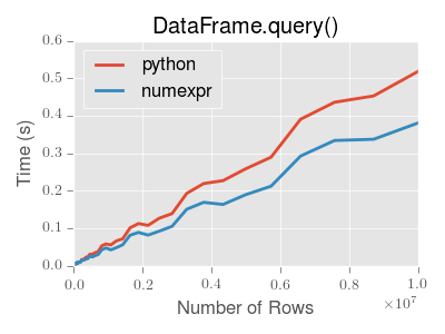
::: tip Note

You will only see the performance benefits of using the numexpr engine with DataFrame.query() if your frame has more than approximately 200,000 rows.

query-perf-small

:::

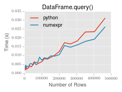
This plot was created using a DataFrame with 3 columns each containing floating point values generated using numpy.random.randn().

Duplicate data

If you want to identify and remove duplicate rows in a DataFrame, there are two methods that will help: duplicated and drop_duplicates. Each takes as an argument the columns to use to identify duplicated rows.

duplicated returns a boolean vector whose length is the number of rows, and which indicates whether a row is duplicated.
drop_duplicates removes duplicate rows.

By default, the first observed row of a duplicate set is considered unique, but each method has a keep parameter to specify targets to be kept.

keep='first' (default): mark / drop duplicates except for the first occurrence.
keep='last': mark / drop duplicates except for the last occurrence.
keep=False: mark / drop all duplicates.

In [264]: df2 = pd.DataFrame({'a': ['one', 'one', 'two', 'two', 'two', 'three', 'four'],
   .....:                     'b': ['x', 'y', 'x', 'y', 'x', 'x', 'x'],
   .....:                     'c': np.random.randn(7)})
   .....: 
In [265]: df2
Out[265]: 
       a  b         c
0    one  x -1.067137
1    one  y  0.309500
2    two  x -0.211056
3    two  y -1.842023
4    two  x -0.390820
5  three  x -1.964475
6   four  x  1.298329
In [266]: df2.duplicated('a')
Out[266]: 
0    False
1     True
2    False
3     True
4     True
5    False
6    False
dtype: bool
In [267]: df2.duplicated('a', keep='last')
Out[267]: 
0     True
1    False
2     True
3     True
4    False
5    False
6    False
dtype: bool
In [268]: df2.duplicated('a', keep=False)
Out[268]: 
0     True
1     True
2     True
3     True
4     True
5    False
6    False
dtype: bool
In [269]: df2.drop_duplicates('a')
Out[269]: 
       a  b         c
0    one  x -1.067137
2    two  x -0.211056
5  three  x -1.964475
6   four  x  1.298329
In [270]: df2.drop_duplicates('a', keep='last')
Out[270]: 
       a  b         c
1    one  y  0.309500
4    two  x -0.390820
5  three  x -1.964475
6   four  x  1.298329
In [271]: df2.drop_duplicates('a', keep=False)
Out[271]: 
       a  b         c
5  three  x -1.964475
6   four  x  1.298329

Also, you can pass a list of columns to identify duplications.

In [272]: df2.duplicated(['a', 'b'])
Out[272]: 
0    False
1    False
2    False
3    False
4     True
5    False
6    False
dtype: bool
In [273]: df2.drop_duplicates(['a', 'b'])
Out[273]: 
       a  b         c
0    one  x -1.067137
1    one  y  0.309500
2    two  x -0.211056
3    two  y -1.842023
5  three  x -1.964475
6   four  x  1.298329

To drop duplicates by index value, use Index.duplicated then perform slicing. The same set of options are available for the keep parameter.

In [274]: df3 = pd.DataFrame({'a': np.arange(6),
   .....:                     'b': np.random.randn(6)},
   .....:                    index=['a', 'a', 'b', 'c', 'b', 'a'])
   .....: 
In [275]: df3
Out[275]: 
   a         b
a  0  1.440455
a  1  2.456086
b  2  1.038402
c  3 -0.894409
b  4  0.683536
a  5  3.082764
In [276]: df3.index.duplicated()
Out[276]: array([False,  True, False, False,  True,  True])
In [277]: df3[~df3.index.duplicated()]
Out[277]: 
   a         b
a  0  1.440455
b  2  1.038402
c  3 -0.894409
In [278]: df3[~df3.index.duplicated(keep='last')]
Out[278]: 
   a         b
c  3 -0.894409
b  4  0.683536
a  5  3.082764
In [279]: df3[~df3.index.duplicated(keep=False)]
Out[279]: 
   a         b
c  3 -0.894409

Dictionary-like `get()` method

Each of Series or DataFrame have a get method which can return a default value.

In [280]: s = pd.Series([1, 2, 3], index=['a', 'b', 'c'])
In [281]: s.get('a')  # equivalent to s['a']
Out[281]: 1
In [282]: s.get('x', default=-1)
Out[282]: -1

The `lookup()` method

Sometimes you want to extract a set of values given a sequence of row labels and column labels, and the lookup method allows for this and returns a NumPy array. For instance:

In [283]: dflookup = pd.DataFrame(np.random.rand(20, 4), columns = ['A', 'B', 'C', 'D'])
In [284]: dflookup.lookup(list(range(0, 10, 2)), ['B', 'C', 'A', 'B', 'D'])
Out[284]: array([0.3506, 0.4779, 0.4825, 0.9197, 0.5019])

Index objects

The pandas Index class and its subclasses can be viewed as implementing an ordered multiset. Duplicates are allowed. However, if you try to convert an Index object with duplicate entries into a set, an exception will be raised.

Index also provides the infrastructure necessary for lookups, data alignment, and reindexing. The easiest way to create an Index directly is to pass a list or other sequence to Index:

In [285]: index = pd.Index(['e', 'd', 'a', 'b'])
In [286]: index
Out[286]: Index(['e', 'd', 'a', 'b'], dtype='object')
In [287]: 'd' in index
Out[287]: True

You can also pass a name to be stored in the index:

In [288]: index = pd.Index(['e', 'd', 'a', 'b'], name='something')
In [289]: index.name
Out[289]: 'something'

The name, if set, will be shown in the console display:

In [290]: index = pd.Index(list(range(5)), name='rows')
In [291]: columns = pd.Index(['A', 'B', 'C'], name='cols')
In [292]: df = pd.DataFrame(np.random.randn(5, 3), index=index, columns=columns)
In [293]: df
Out[293]: 
cols         A         B         C
rows                              
0     1.295989  0.185778  0.436259
1     0.678101  0.311369 -0.528378
2    -0.674808 -1.103529 -0.656157
3     1.889957  2.076651 -1.102192
4    -1.211795 -0.791746  0.634724
In [294]: df['A']
Out[294]: 
rows
0    1.295989
1    0.678101
2   -0.674808
3    1.889957
4   -1.211795
Name: A, dtype: float64

Setting metadata

Indexes are “mostly immutable”, but it is possible to set and change their metadata, like the index name (or, for MultiIndex, levels and codes).

You can use the rename, set_names, set_levels, and set_codes to set these attributes directly. They default to returning a copy; however, you can specify inplace=True to have the data change in place.

See Advanced Indexing for usage of MultiIndexes.

In [295]: ind = pd.Index([1, 2, 3])
In [296]: ind.rename("apple")
Out[296]: Int64Index([1, 2, 3], dtype='int64', name='apple')
In [297]: ind
Out[297]: Int64Index([1, 2, 3], dtype='int64')
In [298]: ind.set_names(["apple"], inplace=True)
In [299]: ind.name = "bob"
In [300]: ind
Out[300]: Int64Index([1, 2, 3], dtype='int64', name='bob')

set_names, set_levels, and set_codes also take an optional level argument

In [301]: index = pd.MultiIndex.from_product([range(3), ['one', 'two']], names=['first', 'second'])
In [302]: index
Out[302]: 
MultiIndex([(0, 'one'),
            (0, 'two'),
            (1, 'one'),
            (1, 'two'),
            (2, 'one'),
            (2, 'two')],
           names=['first', 'second'])
In [303]: index.levels[1]
Out[303]: Index(['one', 'two'], dtype='object', name='second')
In [304]: index.set_levels(["a", "b"], level=1)
Out[304]: 
MultiIndex([(0, 'a'),
            (0, 'b'),
            (1, 'a'),
            (1, 'b'),
            (2, 'a'),
            (2, 'b')],
           names=['first', 'second'])

Set operations on Index objects

The two main operations are union (|) and intersection (&). These can be directly called as instance methods or used via overloaded operators. Difference is provided via the .difference() method.

In [305]: a = pd.Index(['c', 'b', 'a'])
In [306]: b = pd.Index(['c', 'e', 'd'])
In [307]: a | b
Out[307]: Index(['a', 'b', 'c', 'd', 'e'], dtype='object')
In [308]: a & b
Out[308]: Index(['c'], dtype='object')
In [309]: a.difference(b)
Out[309]: Index(['a', 'b'], dtype='object')

Also available is the symmetric_difference (^) operation, which returns elements that appear in either idx1 or idx2, but not in both. This is equivalent to the Index created by idx1.difference(idx2).union(idx2.difference(idx1)), with duplicates dropped.

In [310]: idx1 = pd.Index([1, 2, 3, 4])
In [311]: idx2 = pd.Index([2, 3, 4, 5])
In [312]: idx1.symmetric_difference(idx2)
Out[312]: Int64Index([1, 5], dtype='int64')
In [313]: idx1 ^ idx2
Out[313]: Int64Index([1, 5], dtype='int64')

::: tip Note

The resulting index from a set operation will be sorted in ascending order.

:::

When performing Index.union() between indexes with different dtypes, the indexes must be cast to a common dtype. Typically, though not always, this is object dtype. The exception is when performing a union between integer and float data. In this case, the integer values are converted to float

In [314]: idx1 = pd.Index([0, 1, 2])
In [315]: idx2 = pd.Index([0.5, 1.5])
In [316]: idx1 | idx2
Out[316]: Float64Index([0.0, 0.5, 1.0, 1.5, 2.0], dtype='float64')

Missing values

Even though Index can hold missing values (NaN), it should be avoided if you do not want any unexpected results. For example, some operations exclude missing values implicitly.

Index.fillna fills missing values with specified scalar value.

In [317]: idx1 = pd.Index([1, np.nan, 3, 4])
In [318]: idx1
Out[318]: Float64Index([1.0, nan, 3.0, 4.0], dtype='float64')
In [319]: idx1.fillna(2)
Out[319]: Float64Index([1.0, 2.0, 3.0, 4.0], dtype='float64')
In [320]: idx2 = pd.DatetimeIndex([pd.Timestamp('2011-01-01'),
   .....:                          pd.NaT,
   .....:                          pd.Timestamp('2011-01-03')])
   .....: 
In [321]: idx2
Out[321]: DatetimeIndex(['2011-01-01', 'NaT', '2011-01-03'], dtype='datetime64[ns]', freq=None)
In [322]: idx2.fillna(pd.Timestamp('2011-01-02'))
Out[322]: DatetimeIndex(['2011-01-01', '2011-01-02', '2011-01-03'], dtype='datetime64[ns]', freq=None)

Set / reset index

Occasionally you will load or create a data set into a DataFrame and want to add an index after you’ve already done so. There are a couple of different ways.

Set an index

DataFrame has a set_index() method which takes a column name (for a regular Index) or a list of column names (for a MultiIndex). To create a new, re-indexed DataFrame:

In [323]: data
Out[323]: 
     a    b  c    d
0  bar  one  z  1.0
1  bar  two  y  2.0
2  foo  one  x  3.0
3  foo  two  w  4.0
In [324]: indexed1 = data.set_index('c')
In [325]: indexed1
Out[325]: 
     a    b    d
c               
z  bar  one  1.0
y  bar  two  2.0
x  foo  one  3.0
w  foo  two  4.0
In [326]: indexed2 = data.set_index(['a', 'b'])
In [327]: indexed2
Out[327]: 
         c    d
a   b          
bar one  z  1.0
    two  y  2.0
foo one  x  3.0
    two  w  4.0

The append keyword option allow you to keep the existing index and append the given columns to a MultiIndex:

In [328]: frame = data.set_index('c', drop=False)
In [329]: frame = frame.set_index(['a', 'b'], append=True)
In [330]: frame
Out[330]: 
           c    d
c a   b          
z bar one  z  1.0
y bar two  y  2.0
x foo one  x  3.0
w foo two  w  4.0

Other options in set_index allow you not drop the index columns or to add the index in-place (without creating a new object):

In [331]: data.set_index('c', drop=False)
Out[331]: 
     a    b  c    d
c                  
z  bar  one  z  1.0
y  bar  two  y  2.0
x  foo  one  x  3.0
w  foo  two  w  4.0
In [332]: data.set_index(['a', 'b'], inplace=True)
In [333]: data
Out[333]: 
         c    d
a   b          
bar one  z  1.0
    two  y  2.0
foo one  x  3.0
    two  w  4.0

Reset the index

As a convenience, there is a new function on DataFrame called reset_index() which transfers the index values into the DataFrame’s columns and sets a simple integer index. This is the inverse operation of set_index().

In [334]: data
Out[334]: 
         c    d
a   b          
bar one  z  1.0
    two  y  2.0
foo one  x  3.0
    two  w  4.0
In [335]: data.reset_index()
Out[335]: 
     a    b  c    d
0  bar  one  z  1.0
1  bar  two  y  2.0
2  foo  one  x  3.0
3  foo  two  w  4.0

The output is more similar to a SQL table or a record array. The names for the columns derived from the index are the ones stored in the names attribute.

You can use the level keyword to remove only a portion of the index:

In [336]: frame
Out[336]: 
           c    d
c a   b          
z bar one  z  1.0
y bar two  y  2.0
x foo one  x  3.0
w foo two  w  4.0
In [337]: frame.reset_index(level=1)
Out[337]: 
         a  c    d
c b               
z one  bar  z  1.0
y two  bar  y  2.0
x one  foo  x  3.0
w two  foo  w  4.0

reset_index takes an optional parameter drop which if true simply discards the index, instead of putting index values in the DataFrame’s columns.

Adding an ad hoc index

If you create an index yourself, you can just assign it to the index field:

data.index = index

Returning a view versus a copy

When setting values in a pandas object, care must be taken to avoid what is called chained indexing. Here is an example.

In [338]: dfmi = pd.DataFrame([list('abcd'),
   .....:                      list('efgh'),
   .....:                      list('ijkl'),
   .....:                      list('mnop')],
   .....:                     columns=pd.MultiIndex.from_product([['one', 'two'],
   .....:                                                         ['first', 'second']]))
   .....: 
In [339]: dfmi
Out[339]: 
    one          two       
  first second first second
0     a      b     c      d
1     e      f     g      h
2     i      j     k      l
3     m      n     o      p

Compare these two access methods:

In [340]: dfmi['one']['second']
Out[340]: 
0    b
1    f
2    j
3    n
Name: second, dtype: object

In [341]: dfmi.loc[:, ('one', 'second')]
Out[341]: 
0    b
1    f
2    j
3    n
Name: (one, second), dtype: object

These both yield the same results, so which should you use? It is instructive to understand the order of operations on these and why method 2 (.loc) is much preferred over method 1 (chained []).

dfmi['one'] selects the first level of the columns and returns a DataFrame that is singly-indexed. Then another Python operation dfmi_with_one['second'] selects the series indexed by 'second'. This is indicated by the variable dfmi_with_one because pandas sees these operations as separate events. e.g. separate calls to __getitem__, so it has to treat them as linear operations, they happen one after another.

Contrast this to df.loc[:,('one','second')] which passes a nested tuple of (slice(None),('one','second')) to a single call to __getitem__. This allows pandas to deal with this as a single entity. Furthermore this order of operations can be significantly faster, and allows one to index both axes if so desired.

Why does assignment fail when using chained indexing?

The problem in the previous section is just a performance issue. What’s up with the SettingWithCopy warning? We don’t usually throw warnings around when you do something that might cost a few extra milliseconds!

But it turns out that assigning to the product of chained indexing has inherently unpredictable results. To see this, think about how the Python interpreter executes this code:

dfmi.loc[:, ('one', 'second')] = value
# becomes
dfmi.loc.__setitem__((slice(None), ('one', 'second')), value)

But this code is handled differently:

dfmi['one']['second'] = value
# becomes
dfmi.__getitem__('one').__setitem__('second', value)

See that __getitem__ in there? Outside of simple cases, it’s very hard to predict whether it will return a view or a copy (it depends on the memory layout of the array, about which pandas makes no guarantees), and therefore whether the __setitem__ will modify dfmi or a temporary object that gets thrown out immediately afterward. That’s what SettingWithCopy is warning you about!

::: tip Note

You may be wondering whether we should be concerned about the loc property in the first example. But dfmi.loc is guaranteed to be dfmi itself with modified indexing behavior, so dfmi.loc.__getitem__ / dfmi.loc.__setitem__ operate on dfmi directly. Of course, dfmi.loc.__getitem__(idx) may be a view or a copy of dfmi.

:::

Sometimes a SettingWithCopy warning will arise at times when there’s no obvious chained indexing going on. These are the bugs that SettingWithCopy is designed to catch! Pandas is probably trying to warn you that you’ve done this:

def do_something(df):
    foo = df[['bar', 'baz']]  # Is foo a view? A copy? Nobody knows!
    # ... many lines here ...
    # We don't know whether this will modify df or not!
    foo['quux'] = value
    return foo

Yikes!

Evaluation order matters

When you use chained indexing, the order and type of the indexing operation partially determine whether the result is a slice into the original object, or a copy of the slice.

Pandas has the SettingWithCopyWarning because assigning to a copy of a slice is frequently not intentional, but a mistake caused by chained indexing returning a copy where a slice was expected.

If you would like pandas to be more or less trusting about assignment to a chained indexing expression, you can set the option mode.chained_assignment to one of these values:

'warn', the default, means a SettingWithCopyWarning is printed.
'raise' means pandas will raise a SettingWithCopyException you have to deal with.
None will suppress the warnings entirely.

In [342]: dfb = pd.DataFrame({'a': ['one', 'one', 'two',
   .....:                           'three', 'two', 'one', 'six'],
   .....:                     'c': np.arange(7)})
   .....: 
# This will show the SettingWithCopyWarning
# but the frame values will be set
In [343]: dfb['c'][dfb.a.str.startswith('o')] = 42

This however is operating on a copy and will not work.

>>> pd.set_option('mode.chained_assignment','warn')
>>> dfb[dfb.a.str.startswith('o')]['c'] = 42
Traceback (most recent call last)
     ...
SettingWithCopyWarning:
     A value is trying to be set on a copy of a slice from a DataFrame.
     Try using .loc[row_index,col_indexer] = value instead

A chained assignment can also crop up in setting in a mixed dtype frame.

::: tip Note

These setting rules apply to all of .loc/.iloc.

:::

This is the correct access method:

In [344]: dfc = pd.DataFrame({'A': ['aaa', 'bbb', 'ccc'], 'B': [1, 2, 3]})
In [345]: dfc.loc[0, 'A'] = 11
In [346]: dfc
Out[346]: 
     A  B
0   11  1
1  bbb  2
2  ccc  3

This can work at times, but it is not guaranteed to, and therefore should be avoided:

In [347]: dfc = dfc.copy()
In [348]: dfc['A'][0] = 111
In [349]: dfc
Out[349]: 
     A  B
0  111  1
1  bbb  2
2  ccc  3

This will not work at all, and so should be avoided:

>>> pd.set_option('mode.chained_assignment','raise')
>>> dfc.loc[0]['A'] = 1111
Traceback (most recent call last)
     ...
SettingWithCopyException:
     A value is trying to be set on a copy of a slice from a DataFrame.
     Try using .loc[row_index,col_indexer] = value instead

::: danger Warning

The chained assignment warnings / exceptions are aiming to inform the user of a possibly invalid assignment. There may be false positives; situations where a chained assignment is inadvertently reported.

:::

Indexing and selecting data

Indexing and selecting data

Different choices for indexing

Basics

Attribute access

Slicing ranges

Selection by label

Slicing with labels

Selection by position

Selection by callable

IX indexer is deprecated

Indexing with list with missing labels is deprecated

Reindexing

Selecting random samples

Setting with enlargement

Fast scalar value getting and setting

Boolean indexing

Indexing with isin

The where() Method and Masking

Mask

The query() Method

MultiIndex query() Syntax

query() Use Cases

query() Python versus pandas Syntax Comparison

The in and not in operators

Special use of the == operator with list objects

Boolean operators

Performance of query()

Duplicate data

Dictionary-like get() method

The lookup() method

Index objects

Setting metadata

Set operations on Index objects

Missing values

Set / reset index

Set an index

Reset the index

Adding an ad hoc index

Returning a view versus a copy

Why does assignment fail when using chained indexing?

Evaluation order matters

The `where()` Method and Masking

The `query()` Method

`MultiIndex` `query()` Syntax

`query()` Use Cases

`query()` Python versus pandas Syntax Comparison

The `in` and `not in` operators

Special use of the `==` operator with `list` objects

Performance of `query()`

Dictionary-like `get()` method

The `lookup()` method