烹饪指南

烹饪指南

本节列出了一些短小精悍的 Pandas 实例与链接。

我们希望 Pandas 用户能积极踊跃地为本文档添加更多内容。为本节添加实用示例的链接或代码，是 Pandas 用户提交第一个 Pull Request 最好的选择。

本节列出了简单、精练、易上手的实例代码，以及 Stack Overflow 或 GitHub 上的链接，这些链接包含实例代码的更多详情。

pd 与 np 是 Pandas 与 Numpy 的缩写。为了让新手易于理解，其它模块是显式导入的。

下列实例均为 Python 3 代码，简单修改即可用于 Python 早期版本。

惯用语

以下是 Pandas 的惯用语。

对一列数据执行 if-then / if-then-else 操作，把计算结果赋值给一列或多列：

In [1]: df = pd.DataFrame({'AAA': [4, 5, 6, 7],
   ...:                    'BBB': [10, 20, 30, 40],
   ...:                    'CCC': [100, 50, -30, -50]})
   ...: 
In [2]: df
Out[2]: 
   AAA  BBB  CCC
0    4   10  100
1    5   20   50
2    6   30  -30
3    7   40  -50

if-then…

在一列上执行 if-then 操作：

In [3]: df.loc[df.AAA >= 5, 'BBB'] = -1
In [4]: df
Out[4]: 
   AAA  BBB  CCC
0    4   10  100
1    5   -1   50
2    6   -1  -30
3    7   -1  -50

在两列上执行 if-then 操作：

In [5]: df.loc[df.AAA >= 5, ['BBB', 'CCC']] = 555
In [6]: df
Out[6]: 
   AAA  BBB  CCC
0    4   10  100
1    5  555  555
2    6  555  555
3    7  555  555

再添加一行代码，执行 -else 操作：

In [7]: df.loc[df.AAA < 5, ['BBB', 'CCC']] = 2000
In [8]: df
Out[8]: 
   AAA   BBB   CCC
0    4  2000  2000
1    5   555   555
2    6   555   555
3    7   555   555

或用 Pandas 的 where 设置掩码（mask）：

In [9]: df_mask = pd.DataFrame({'AAA': [True] * 4,
   ...:                         'BBB': [False] * 4,
   ...:                         'CCC': [True, False] * 2})
   ...: 
In [10]: df.where(df_mask, -1000)
Out[10]: 
   AAA   BBB   CCC
0    4 -1000  2000
1    5 -1000 -1000
2    6 -1000   555
3    7 -1000 -1000

用 NumPy where() 函数实现 if-then-else

In [11]: df = pd.DataFrame({'AAA': [4, 5, 6, 7],
   ....:                    'BBB': [10, 20, 30, 40],
   ....:                    'CCC': [100, 50, -30, -50]})
   ....: 
In [12]: df
Out[12]: 
   AAA  BBB  CCC
0    4   10  100
1    5   20   50
2    6   30  -30
3    7   40  -50
In [13]: df['logic'] = np.where(df['AAA'] > 5, 'high', 'low')
In [14]: df
Out[14]: 
   AAA  BBB  CCC logic
0    4   10  100   low
1    5   20   50   low
2    6   30  -30  high
3    7   40  -50  high

切割

用布尔条件切割 DataFrame

In [15]: df = pd.DataFrame({'AAA': [4, 5, 6, 7],
   ....:                    'BBB': [10, 20, 30, 40],
   ....:                    'CCC': [100, 50, -30, -50]})
   ....: 
In [16]: df
Out[16]: 
   AAA  BBB  CCC
0    4   10  100
1    5   20   50
2    6   30  -30
3    7   40  -50
In [17]: df[df.AAA <= 5]
Out[17]: 
   AAA  BBB  CCC
0    4   10  100
1    5   20   50
In [18]: df[df.AAA > 5]
Out[18]: 
   AAA  BBB  CCC
2    6   30  -30
3    7   40  -50

设置条件

多列条件选择

In [19]: df = pd.DataFrame({'AAA': [4, 5, 6, 7],
   ....:                    'BBB': [10, 20, 30, 40],
   ....:                    'CCC': [100, 50, -30, -50]})
   ....: 
In [20]: df
Out[20]: 
   AAA  BBB  CCC
0    4   10  100
1    5   20   50
2    6   30  -30
3    7   40  -50

和（&），不赋值，直接返回 Series：

In [21]: df.loc[(df['BBB'] < 25) & (df['CCC'] >= -40), 'AAA']
Out[21]: 
0    4
1    5
Name: AAA, dtype: int64

或（|），不赋值，直接返回 Series：

In [22]: df.loc[(df['BBB'] > 25) | (df['CCC'] >= -40), 'AAA']
Out[22]: 
0    4
1    5
2    6
3    7
Name: AAA, dtype: int64

或（|），赋值，修改 DataFrame：

In [23]: df.loc[(df['BBB'] > 25) | (df['CCC'] >= 75), 'AAA'] = 0.1
In [24]: df
Out[24]: 
   AAA  BBB  CCC
0  0.1   10  100
1  5.0   20   50
2  0.1   30  -30
3  0.1   40  -50

用 argsort 选择最接近指定值的行

In [25]: df = pd.DataFrame({'AAA': [4, 5, 6, 7],
   ....:                    'BBB': [10, 20, 30, 40],
   ....:                    'CCC': [100, 50, -30, -50]})
   ....: 
In [26]: df
Out[26]: 
   AAA  BBB  CCC
0    4   10  100
1    5   20   50
2    6   30  -30
3    7   40  -50
In [27]: aValue = 43.0
In [28]: df.loc[(df.CCC - aValue).abs().argsort()]
Out[28]: 
   AAA  BBB  CCC
1    5   20   50
0    4   10  100
2    6   30  -30
3    7   40  -50

用二进制运算符动态减少条件列表

In [29]: df = pd.DataFrame({'AAA': [4, 5, 6, 7],
   ....:                    'BBB': [10, 20, 30, 40],
   ....:                    'CCC': [100, 50, -30, -50]})
   ....: 
In [30]: df
Out[30]: 
   AAA  BBB  CCC
0    4   10  100
1    5   20   50
2    6   30  -30
3    7   40  -50
In [31]: Crit1 = df.AAA <= 5.5
In [32]: Crit2 = df.BBB == 10.0
In [33]: Crit3 = df.CCC > -40.0

硬编码方式为：

In [34]: AllCrit = Crit1 & Crit2 & Crit3

生成动态条件列表：

In [35]: import functools
In [36]: CritList = [Crit1, Crit2, Crit3]
In [37]: AllCrit = functools.reduce(lambda x, y: x & y, CritList)
In [38]: df[AllCrit]
Out[38]: 
   AAA  BBB  CCC
0    4   10  100

选择

DataFrames

更多信息，请参阅索引文档。

行标签与值作为条件

In [39]: df = pd.DataFrame({'AAA': [4, 5, 6, 7],
   ....:                    'BBB': [10, 20, 30, 40],
   ....:                    'CCC': [100, 50, -30, -50]})
   ....: 
In [40]: df
Out[40]: 
   AAA  BBB  CCC
0    4   10  100
1    5   20   50
2    6   30  -30
3    7   40  -50
In [41]: df[(df.AAA <= 6) & (df.index.isin([0, 2, 4]))]
Out[41]: 
   AAA  BBB  CCC
0    4   10  100
2    6   30  -30

标签切片用 loc，位置切片用 iloc

In [42]: df = pd.DataFrame({'AAA': [4, 5, 6, 7],
   ....:                    'BBB': [10, 20, 30, 40],
   ....:                    'CCC': [100, 50, -30, -50]},
   ....:                   index=['foo', 'bar', 'boo', 'kar'])
   ....:

前 2 个是显式切片方法，第 3 个是通用方法：

位置切片，Python 切片风格，不包括结尾数据；
标签切片，非 Python 切片风格，包括结尾数据；
通用切片，支持两种切片风格，取决于切片用的是标签还是位置。

In [43]: df.loc['bar':'kar']  # Label
Out[43]: 
     AAA  BBB  CCC
bar    5   20   50
boo    6   30  -30
kar    7   40  -50
# Generic
In [44]: df.iloc[0:3]
Out[44]: 
     AAA  BBB  CCC
foo    4   10  100
bar    5   20   50
boo    6   30  -30
In [45]: df.loc['bar':'kar']
Out[45]: 
     AAA  BBB  CCC
bar    5   20   50
boo    6   30  -30
kar    7   40  -50

包含整数，且不从 0 开始的索引，或不是逐步递增的索引会引发歧义。

In [46]: data = {'AAA': [4, 5, 6, 7],
   ....:         'BBB': [10, 20, 30, 40],
   ....:         'CCC': [100, 50, -30, -50]}
   ....: 
In [47]: df2 = pd.DataFrame(data=data, index=[1, 2, 3, 4])  # Note index starts at 1.
In [48]: df2.iloc[1:3]  # Position-oriented
Out[48]: 
   AAA  BBB  CCC
2    5   20   50
3    6   30  -30
In [49]: df2.loc[1:3]  # Label-oriented
Out[49]: 
   AAA  BBB  CCC
1    4   10  100
2    5   20   50
3    6   30  -30

用逆运算符 (~)提取掩码的反向内容

In [50]: df = pd.DataFrame({'AAA': [4, 5, 6, 7],
   ....:                    'BBB': [10, 20, 30, 40],
   ....:                    'CCC': [100, 50, -30, -50]})
   ....: 
In [51]: df
Out[51]: 
   AAA  BBB  CCC
0    4   10  100
1    5   20   50
2    6   30  -30
3    7   40  -50
In [52]: df[~((df.AAA <= 6) & (df.index.isin([0, 2, 4])))]
Out[52]: 
   AAA  BBB  CCC
1    5   20   50
3    7   40  -50

生成新列

用 applymap 高效动态生成新列

In [53]: df = pd.DataFrame({'AAA': [1, 2, 1, 3],
   ....:                    'BBB': [1, 1, 2, 2],
   ....:                    'CCC': [2, 1, 3, 1]})
   ....: 
In [54]: df
Out[54]: 
   AAA  BBB  CCC
0    1    1    2
1    2    1    1
2    1    2    3
3    3    2    1
In [55]: source_cols = df.columns   # Or some subset would work too
In [56]: new_cols = [str(x) + "_cat" for x in source_cols]
In [57]: categories = {1: 'Alpha', 2: 'Beta', 3: 'Charlie'}
In [58]: df[new_cols] = df[source_cols].applymap(categories.get)
In [59]: df
Out[59]: 
   AAA  BBB  CCC  AAA_cat BBB_cat  CCC_cat
0    1    1    2    Alpha   Alpha     Beta
1    2    1    1     Beta   Alpha    Alpha
2    1    2    3    Alpha    Beta  Charlie
3    3    2    1  Charlie    Beta    Alpha

分组时用 min()

In [60]: df = pd.DataFrame({'AAA': [1, 1, 1, 2, 2, 2, 3, 3],
   ....:                    'BBB': [2, 1, 3, 4, 5, 1, 2, 3]})
   ....: 
In [61]: df
Out[61]: 
   AAA  BBB
0    1    2
1    1    1
2    1    3
3    2    4
4    2    5
5    2    1
6    3    2
7    3    3

方法1：用 idxmin() 提取每组最小值的索引

In [62]: df.loc[df.groupby("AAA")["BBB"].idxmin()]
Out[62]: 
   AAA  BBB
1    1    1
5    2    1
6    3    2

方法 2：先排序，再提取每组的第一个值

In [63]: df.sort_values(by="BBB").groupby("AAA", as_index=False).first()
Out[63]: 
   AAA  BBB
0    1    1
1    2    1
2    3    2

注意，提取的数据一样，但索引不一样。

多层索引

更多信息，请参阅多层索引文档。

用带标签的字典创建多层索引

In [64]: df = pd.DataFrame({'row': [0, 1, 2],
   ....:                    'One_X': [1.1, 1.1, 1.1],
   ....:                    'One_Y': [1.2, 1.2, 1.2],
   ....:                    'Two_X': [1.11, 1.11, 1.11],
   ....:                    'Two_Y': [1.22, 1.22, 1.22]})
   ....: 
In [65]: df
Out[65]: 
   row  One_X  One_Y  Two_X  Two_Y
0    0    1.1    1.2   1.11   1.22
1    1    1.1    1.2   1.11   1.22
2    2    1.1    1.2   1.11   1.22
# 设置索引标签
In [66]: df = df.set_index('row')
In [67]: df
Out[67]: 
     One_X  One_Y  Two_X  Two_Y
row                            
0      1.1    1.2   1.11   1.22
1      1.1    1.2   1.11   1.22
2      1.1    1.2   1.11   1.22
# 多层索引的列
In [68]: df.columns = pd.MultiIndex.from_tuples([tuple(c.split('_'))
   ....:                                         for c in df.columns])
   ....: 
In [69]: df
Out[69]: 
     One        Two      
       X    Y     X     Y
row                      
0    1.1  1.2  1.11  1.22
1    1.1  1.2  1.11  1.22
2    1.1  1.2  1.11  1.22
# 先 stack，然后 Reset 索引
In [70]: df = df.stack(0).reset_index(1)
In [71]: df
Out[71]: 
    level_1     X     Y
row                    
0       One  1.10  1.20
0       Two  1.11  1.22
1       One  1.10  1.20
1       Two  1.11  1.22
2       One  1.10  1.20
2       Two  1.11  1.22
# 修整标签，注意自动添加了标签 `level_1` 
In [72]: df.columns = ['Sample', 'All_X', 'All_Y']
In [73]: df
Out[73]: 
    Sample  All_X  All_Y
row                     
0      One   1.10   1.20
0      Two   1.11   1.22
1      One   1.10   1.20
1      Two   1.11   1.22
2      One   1.10   1.20
2      Two   1.11   1.22

运算

多层索引运算要用广播机制

In [74]: cols = pd.MultiIndex.from_tuples([(x, y) for x in ['A', 'B', 'C']
   ....:                                   for y in ['O', 'I']])
   ....: 
In [75]: df = pd.DataFrame(np.random.randn(2, 6), index=['n', 'm'], columns=cols)
In [76]: df
Out[76]: 
          A                   B                   C          
          O         I         O         I         O         I
n  0.469112 -0.282863 -1.509059 -1.135632  1.212112 -0.173215
m  0.119209 -1.044236 -0.861849 -2.104569 -0.494929  1.071804
In [77]: df = df.div(df['C'], level=1)
In [78]: df
Out[78]: 
          A                   B              C     
          O         I         O         I    O    I
n  0.387021  1.633022 -1.244983  6.556214  1.0  1.0
m -0.240860 -0.974279  1.741358 -1.963577  1.0  1.0

切片

用 xs 切片多层索引

In [79]: coords = [('AA', 'one'), ('AA', 'six'), ('BB', 'one'), ('BB', 'two'),
   ....:           ('BB', 'six')]
   ....: 
In [80]: index = pd.MultiIndex.from_tuples(coords)
In [81]: df = pd.DataFrame([11, 22, 33, 44, 55], index, ['MyData'])
In [82]: df
Out[82]: 
        MyData
AA one      11
   six      22
BB one      33
   two      44
   six      55

提取第一层与索引第一个轴的交叉数据：

# 注意：level 与 axis 是可选项，默认为 0
In [83]: df.xs('BB', level=0, axis=0)
Out[83]: 
     MyData
one      33
two      44
six      55

……现在是第 1 个轴的第 2 层

In [84]: df.xs('six', level=1, axis=0)
Out[84]: 
    MyData
AA      22
BB      55

用 xs 切片多层索引，方法 #2

In [85]: import itertools
In [86]: index = list(itertools.product(['Ada', 'Quinn', 'Violet'],
   ....:                                ['Comp', 'Math', 'Sci']))
   ....: 
In [87]: headr = list(itertools.product(['Exams', 'Labs'], ['I', 'II']))
In [88]: indx = pd.MultiIndex.from_tuples(index, names=['Student', 'Course'])
In [89]: cols = pd.MultiIndex.from_tuples(headr)   # Notice these are un-named
In [90]: data = [[70 + x + y + (x * y) % 3 for x in range(4)] for y in range(9)]
In [91]: df = pd.DataFrame(data, indx, cols)
In [92]: df
Out[92]: 
               Exams     Labs    
                   I  II    I  II
Student Course                   
Ada     Comp      70  71   72  73
        Math      71  73   75  74
        Sci       72  75   75  75
Quinn   Comp      73  74   75  76
        Math      74  76   78  77
        Sci       75  78   78  78
Violet  Comp      76  77   78  79
        Math      77  79   81  80
        Sci       78  81   81  81
In [93]: All = slice(None)
In [94]: df.loc['Violet']
Out[94]: 
       Exams     Labs    
           I  II    I  II
Course                   
Comp      76  77   78  79
Math      77  79   81  80
Sci       78  81   81  81
In [95]: df.loc[(All, 'Math'), All]
Out[95]: 
               Exams     Labs    
                   I  II    I  II
Student Course                   
Ada     Math      71  73   75  74
Quinn   Math      74  76   78  77
Violet  Math      77  79   81  80
In [96]: df.loc[(slice('Ada', 'Quinn'), 'Math'), All]
Out[96]: 
               Exams     Labs    
                   I  II    I  II
Student Course                   
Ada     Math      71  73   75  74
Quinn   Math      74  76   78  77
In [97]: df.loc[(All, 'Math'), ('Exams')]
Out[97]: 
                 I  II
Student Course        
Ada     Math    71  73
Quinn   Math    74  76
Violet  Math    77  79
In [98]: df.loc[(All, 'Math'), (All, 'II')]
Out[98]: 
               Exams Labs
                  II   II
Student Course           
Ada     Math      73   74
Quinn   Math      76   77
Violet  Math      79   80

用 xs 设置多层索引比例

排序

用多层索引按指定列或列序列表排序x

In [99]: df.sort_values(by=('Labs', 'II'), ascending=False)
Out[99]: 
               Exams     Labs    
                   I  II    I  II
Student Course                   
Violet  Sci       78  81   81  81
        Math      77  79   81  80
        Comp      76  77   78  79
Quinn   Sci       75  78   78  78
        Math      74  76   78  77
        Comp      73  74   75  76
Ada     Sci       72  75   75  75
        Math      71  73   75  74
        Comp      70  71   72  73

部分选择，需要排序

层级

为多层索引添加一层

平铺结构化列

缺失数据

缺失数据文档。

向前填充逆序时间序列。

In [100]: df = pd.DataFrame(np.random.randn(6, 1),
   .....:                   index=pd.date_range('2013-08-01', periods=6, freq='B'),
   .....:                   columns=list('A'))
   .....: 
In [101]: df.loc[df.index[3], 'A'] = np.nan
In [102]: df
Out[102]: 
                   A
2013-08-01  0.721555
2013-08-02 -0.706771
2013-08-05 -1.039575
2013-08-06       NaN
2013-08-07 -0.424972
2013-08-08  0.567020
In [103]: df.reindex(df.index[::-1]).ffill()
Out[103]: 
                   A
2013-08-08  0.567020
2013-08-07 -0.424972
2013-08-06 -0.424972
2013-08-05 -1.039575
2013-08-02 -0.706771
2013-08-01  0.721555

空值时重置为 0，有值时累加

替换

用反引用替换

分组

分组文档。

用 apply 执行分组基础操作

与聚合不同，传递给 DataFrame 子集的 apply 可回调，可以访问所有列。

In [104]: df = pd.DataFrame({'animal': 'cat dog cat fish dog cat cat'.split(),
   .....:                    'size': list('SSMMMLL'),
   .....:                    'weight': [8, 10, 11, 1, 20, 12, 12],
   .....:                    'adult': [False] * 5 + [True] * 2})
   .....: 
In [105]: df
Out[105]: 
  animal size  weight  adult
0    cat    S       8  False
1    dog    S      10  False
2    cat    M      11  False
3   fish    M       1  False
4    dog    M      20  False
5    cat    L      12   True
6    cat    L      12   True
# 提取 size 列最重的动物列表
In [106]: df.groupby('animal').apply(lambda subf: subf['size'][subf['weight'].idxmax()])
Out[106]: 
animal
cat     L
dog     M
fish    M
dtype: object

使用 get_group

In [107]: gb = df.groupby(['animal'])
In [108]: gb.get_group('cat')
Out[108]: 
  animal size  weight  adult
0    cat    S       8  False
2    cat    M      11  False
5    cat    L      12   True
6    cat    L      12   True

为同一分组的不同内容使用 Apply 函数

In [109]: def GrowUp(x):
   .....:     avg_weight = sum(x[x['size'] == 'S'].weight * 1.5)
   .....:     avg_weight += sum(x[x['size'] == 'M'].weight * 1.25)
   .....:     avg_weight += sum(x[x['size'] == 'L'].weight)
   .....:     avg_weight /= len(x)
   .....:     return pd.Series(['L', avg_weight, True],
   .....:                      index=['size', 'weight', 'adult'])
   .....: 
In [110]: expected_df = gb.apply(GrowUp)
In [111]: expected_df
Out[111]: 
       size   weight  adult
animal                     
cat       L  12.4375   True
dog       L  20.0000   True
fish      L   1.2500   True

Apply 函数扩展

In [112]: S = pd.Series([i / 100.0 for i in range(1, 11)])
In [113]: def cum_ret(x, y):
   .....:     return x * (1 + y)
   .....: 
In [114]: def red(x):
   .....:     return functools.reduce(cum_ret, x, 1.0)
   .....: 
In [115]: S.expanding().apply(red, raw=True)
Out[115]: 
0    1.010000
1    1.030200
2    1.061106
3    1.103550
4    1.158728
5    1.228251
6    1.314229
7    1.419367
8    1.547110
9    1.701821
dtype: float64

用分组里的剩余值的平均值进行替换

In [116]: df = pd.DataFrame({'A': [1, 1, 2, 2], 'B': [1, -1, 1, 2]})
In [117]: gb = df.groupby('A')
In [118]: def replace(g):
   .....:     mask = g < 0
   .....:     return g.where(mask, g[~mask].mean())
   .....: 
In [119]: gb.transform(replace)
Out[119]: 
     B
0  1.0
1 -1.0
2  1.5
3  1.5

按聚合数据排序

In [120]: df = pd.DataFrame({'code': ['foo', 'bar', 'baz'] * 2,
   .....:                    'data': [0.16, -0.21, 0.33, 0.45, -0.59, 0.62],
   .....:                    'flag': [False, True] * 3})
   .....: 
In [121]: code_groups = df.groupby('code')
In [122]: agg_n_sort_order = code_groups[['data']].transform(sum).sort_values(by='data')
In [123]: sorted_df = df.loc[agg_n_sort_order.index]
In [124]: sorted_df
Out[124]: 
  code  data   flag
1  bar -0.21   True
4  bar -0.59  False
0  foo  0.16  False
3  foo  0.45   True
2  baz  0.33  False
5  baz  0.62   True

创建多个聚合列

In [125]: rng = pd.date_range(start="2014-10-07", periods=10, freq='2min')
In [126]: ts = pd.Series(data=list(range(10)), index=rng)
In [127]: def MyCust(x):
   .....:     if len(x) > 2:
   .....:         return x[1] * 1.234
   .....:     return pd.NaT
   .....: 
In [128]: mhc = {'Mean': np.mean, 'Max': np.max, 'Custom': MyCust}
In [129]: ts.resample("5min").apply(mhc)
Out[129]: 
Mean    2014-10-07 00:00:00        1
        2014-10-07 00:05:00      3.5
        2014-10-07 00:10:00        6
        2014-10-07 00:15:00      8.5
Max     2014-10-07 00:00:00        2
        2014-10-07 00:05:00        4
        2014-10-07 00:10:00        7
        2014-10-07 00:15:00        9
Custom  2014-10-07 00:00:00    1.234
        2014-10-07 00:05:00      NaT
        2014-10-07 00:10:00    7.404
        2014-10-07 00:15:00      NaT
dtype: object
In [130]: ts
Out[130]: 
2014-10-07 00:00:00    0
2014-10-07 00:02:00    1
2014-10-07 00:04:00    2
2014-10-07 00:06:00    3
2014-10-07 00:08:00    4
2014-10-07 00:10:00    5
2014-10-07 00:12:00    6
2014-10-07 00:14:00    7
2014-10-07 00:16:00    8
2014-10-07 00:18:00    9
Freq: 2T, dtype: int64

为 DataFrame 创建值计数列

In [131]: df = pd.DataFrame({'Color': 'Red Red Red Blue'.split(),
   .....:                    'Value': [100, 150, 50, 50]})
   .....: 
In [132]: df
Out[132]: 
  Color  Value
0   Red    100
1   Red    150
2   Red     50
3  Blue     50
In [133]: df['Counts'] = df.groupby(['Color']).transform(len)
In [134]: df
Out[134]: 
  Color  Value  Counts
0   Red    100       3
1   Red    150       3
2   Red     50       3
3  Blue     50       1

基于索引唯一某列不同分组的值

In [135]: df = pd.DataFrame({'line_race': [10, 10, 8, 10, 10, 8],
   .....:                    'beyer': [99, 102, 103, 103, 88, 100]},
   .....:                   index=['Last Gunfighter', 'Last Gunfighter',
   .....:                          'Last Gunfighter', 'Paynter', 'Paynter',
   .....:                          'Paynter'])
   .....: 
In [136]: df
Out[136]: 
                 line_race  beyer
Last Gunfighter         10     99
Last Gunfighter         10    102
Last Gunfighter          8    103
Paynter                 10    103
Paynter                 10     88
Paynter                  8    100
In [137]: df['beyer_shifted'] = df.groupby(level=0)['beyer'].shift(1)
In [138]: df
Out[138]: 
                 line_race  beyer  beyer_shifted
Last Gunfighter         10     99            NaN
Last Gunfighter         10    102           99.0
Last Gunfighter          8    103          102.0
Paynter                 10    103            NaN
Paynter                 10     88          103.0
Paynter                  8    100           88.0

选择每组最大值的行

In [139]: df = pd.DataFrame({'host': ['other', 'other', 'that', 'this', 'this'],
   .....:                    'service': ['mail', 'web', 'mail', 'mail', 'web'],
   .....:                    'no': [1, 2, 1, 2, 1]}).set_index(['host', 'service'])
   .....: 
In [140]: mask = df.groupby(level=0).agg('idxmax')
In [141]: df_count = df.loc[mask['no']].reset_index()
In [142]: df_count
Out[142]: 
    host service  no
0  other     web   2
1   that    mail   1
2   this    mail   2

Python itertools.groupby 式分组

In [143]: df = pd.DataFrame([0, 1, 0, 1, 1, 1, 0, 1, 1], columns=['A'])
In [144]: df.A.groupby((df.A != df.A.shift()).cumsum()).groups
Out[144]: 
{1: Int64Index([0], dtype='int64'),
 2: Int64Index([1], dtype='int64'),
 3: Int64Index([2], dtype='int64'),
 4: Int64Index([3, 4, 5], dtype='int64'),
 5: Int64Index([6], dtype='int64'),
 6: Int64Index([7, 8], dtype='int64')}
In [145]: df.A.groupby((df.A != df.A.shift()).cumsum()).cumsum()
Out[145]: 
0    0
1    1
2    0
3    1
4    2
5    3
6    0
7    1
8    2
Name: A, dtype: int64

扩展数据

Alignment and to-date

基于计数值进行移动窗口计算

按时间间隔计算滚动平均

分割

分割 DataFrame

按指定逻辑，将不同的行，分割成 DataFrame 列表。

In [146]: df = pd.DataFrame(data={'Case': ['A', 'A', 'A', 'B', 'A', 'A', 'B', 'A',
   .....:                                  'A'],
   .....:                         'Data': np.random.randn(9)})
   .....: 
In [147]: dfs = list(zip(*df.groupby((1 * (df['Case'] == 'B')).cumsum()
   .....:                .rolling(window=3, min_periods=1).median())))[-1]
   .....: 
In [148]: dfs[0]
Out[148]: 
  Case      Data
0    A  0.276232
1    A -1.087401
2    A -0.673690
3    B  0.113648
In [149]: dfs[1]
Out[149]: 
  Case      Data
4    A -1.478427
5    A  0.524988
6    B  0.404705
In [150]: dfs[2]
Out[150]: 
  Case      Data
7    A  0.577046
8    A -1.715002

透视表

透视表文档。

部分汇总与小计

In [151]: df = pd.DataFrame(data={'Province': ['ON', 'QC', 'BC', 'AL', 'AL', 'MN', 'ON'],
   .....:                         'City': ['Toronto', 'Montreal', 'Vancouver',
   .....:                                  'Calgary', 'Edmonton', 'Winnipeg',
   .....:                                  'Windsor'],
   .....:                         'Sales': [13, 6, 16, 8, 4, 3, 1]})
   .....: 
In [152]: table = pd.pivot_table(df, values=['Sales'], index=['Province'],
   .....:                        columns=['City'], aggfunc=np.sum, margins=True)
   .....: 
In [153]: table.stack('City')
Out[153]: 
                    Sales
Province City            
AL       All         12.0
         Calgary      8.0
         Edmonton     4.0
BC       All         16.0
         Vancouver   16.0
...                   ...
All      Montreal     6.0
         Toronto     13.0
         Vancouver   16.0
         Windsor      1.0
         Winnipeg     3.0
[20 rows x 1 columns]

类似 R 的 plyr 频率表

In [154]: grades = [48, 99, 75, 80, 42, 80, 72, 68, 36, 78]
In [155]: df = pd.DataFrame({'ID': ["x%d" % r for r in range(10)],
   .....:                    'Gender': ['F', 'M', 'F', 'M', 'F',
   .....:                               'M', 'F', 'M', 'M', 'M'],
   .....:                    'ExamYear': ['2007', '2007', '2007', '2008', '2008',
   .....:                                 '2008', '2008', '2009', '2009', '2009'],
   .....:                    'Class': ['algebra', 'stats', 'bio', 'algebra',
   .....:                              'algebra', 'stats', 'stats', 'algebra',
   .....:                              'bio', 'bio'],
   .....:                    'Participated': ['yes', 'yes', 'yes', 'yes', 'no',
   .....:                                     'yes', 'yes', 'yes', 'yes', 'yes'],
   .....:                    'Passed': ['yes' if x > 50 else 'no' for x in grades],
   .....:                    'Employed': [True, True, True, False,
   .....:                                 False, False, False, True, True, False],
   .....:                    'Grade': grades})
   .....: 
In [156]: df.groupby('ExamYear').agg({'Participated': lambda x: x.value_counts()['yes'],
   .....:                             'Passed': lambda x: sum(x == 'yes'),
   .....:                             'Employed': lambda x: sum(x),
   .....:                             'Grade': lambda x: sum(x) / len(x)})
   .....: 
Out[156]: 
          Participated  Passed  Employed      Grade
ExamYear                                           
2007                 3       2         3  74.000000
2008                 3       3         0  68.500000
2009                 3       2         2  60.666667

按年生成 DataFrame

跨列表创建年月：

In [157]: df = pd.DataFrame({'value': np.random.randn(36)},
   .....:                   index=pd.date_range('2011-01-01', freq='M', periods=36))
   .....: 
In [158]: pd.pivot_table(df, index=df.index.month, columns=df.index.year,
   .....:                values='value', aggfunc='sum')
   .....: 
Out[158]: 
        2011      2012      2013
1  -1.039268 -0.968914  2.565646
2  -0.370647 -1.294524  1.431256
3  -1.157892  0.413738  1.340309
4  -1.344312  0.276662 -1.170299
5   0.844885 -0.472035 -0.226169
6   1.075770 -0.013960  0.410835
7  -0.109050 -0.362543  0.813850
8   1.643563 -0.006154  0.132003
9  -1.469388 -0.923061 -0.827317
10  0.357021  0.895717 -0.076467
11 -0.674600  0.805244 -1.187678
12 -1.776904 -1.206412  1.130127

Apply 函数

把嵌入列表转换为多层索引 DataFrame

In [159]: df = pd.DataFrame(data={'A': [[2, 4, 8, 16], [100, 200], [10, 20, 30]],
   .....:                         'B': [['a', 'b', 'c'], ['jj', 'kk'], ['ccc']]},
   .....:                   index=['I', 'II', 'III'])
   .....: 
In [160]: def SeriesFromSubList(aList):
   .....:     return pd.Series(aList)
   .....: 
In [161]: df_orgz = pd.concat({ind: row.apply(SeriesFromSubList)
   .....:                      for ind, row in df.iterrows()})
   .....: 
In [162]: df_orgz
Out[162]: 
         0    1    2     3
I   A    2    4    8  16.0
    B    a    b    c   NaN
II  A  100  200  NaN   NaN
    B   jj   kk  NaN   NaN
III A   10   20   30   NaN
    B  ccc  NaN  NaN   NaN

返回 Series

Rolling Apply to multiple columns where function calculates a Series before a Scalar from the Series is returned

In [163]: df = pd.DataFrame(data=np.random.randn(2000, 2) / 10000,
   .....:                   index=pd.date_range('2001-01-01', periods=2000),
   .....:                   columns=['A', 'B'])
   .....: 
In [164]: df
Out[164]: 
                   A         B
2001-01-01 -0.000144 -0.000141
2001-01-02  0.000161  0.000102
2001-01-03  0.000057  0.000088
2001-01-04 -0.000221  0.000097
2001-01-05 -0.000201 -0.000041
...              ...       ...
2006-06-19  0.000040 -0.000235
2006-06-20 -0.000123 -0.000021
2006-06-21 -0.000113  0.000114
2006-06-22  0.000136  0.000109
2006-06-23  0.000027  0.000030
[2000 rows x 2 columns]
In [165]: def gm(df, const):
   .....:     v = ((((df.A + df.B) + 1).cumprod()) - 1) * const
   .....:     return v.iloc[-1]
   .....: 
In [166]: s = pd.Series({df.index[i]: gm(df.iloc[i:min(i + 51, len(df) - 1)], 5)
   .....:                for i in range(len(df) - 50)})
   .....: 
In [167]: s
Out[167]: 
2001-01-01    0.000930
2001-01-02    0.002615
2001-01-03    0.001281
2001-01-04    0.001117
2001-01-05    0.002772
                ...   
2006-04-30    0.003296
2006-05-01    0.002629
2006-05-02    0.002081
2006-05-03    0.004247
2006-05-04    0.003928
Length: 1950, dtype: float64

返回标量值

Rolling Apply to multiple columns where function returns a Scalar (Volume Weighted Average Price) 对多列执行滚动 Apply，函数返回标量值（成交价加权平均价）

In [168]: rng = pd.date_range(start='2014-01-01', periods=100)
In [169]: df = pd.DataFrame({'Open': np.random.randn(len(rng)),
   .....:                    'Close': np.random.randn(len(rng)),
   .....:                    'Volume': np.random.randint(100, 2000, len(rng))},
   .....:                   index=rng)
   .....: 
In [170]: df
Out[170]: 
                Open     Close  Volume
2014-01-01 -1.611353 -0.492885    1219
2014-01-02 -3.000951  0.445794    1054
2014-01-03 -0.138359 -0.076081    1381
2014-01-04  0.301568  1.198259    1253
2014-01-05  0.276381 -0.669831    1728
...              ...       ...     ...
2014-04-06 -0.040338  0.937843    1188
2014-04-07  0.359661 -0.285908    1864
2014-04-08  0.060978  1.714814     941
2014-04-09  1.759055 -0.455942    1065
2014-04-10  0.138185 -1.147008    1453
[100 rows x 3 columns]
In [171]: def vwap(bars):
   .....:     return ((bars.Close * bars.Volume).sum() / bars.Volume.sum())
   .....: 
In [172]: window = 5
In [173]: s = pd.concat([(pd.Series(vwap(df.iloc[i:i + window]),
   .....:                 index=[df.index[i + window]]))
   .....:                for i in range(len(df) - window)])
   .....: 
In [174]: s.round(2)
Out[174]: 
2014-01-06    0.02
2014-01-07    0.11
2014-01-08    0.10
2014-01-09    0.07
2014-01-10   -0.29
              ... 
2014-04-06   -0.63
2014-04-07   -0.02
2014-04-08   -0.03
2014-04-09    0.34
2014-04-10    0.29
Length: 95, dtype: float64

时间序列

删除指定时间之外的数据

用 indexer 提取在时间范围内的数据

创建不包括周末，且只包含指定时间的日期时间范围

矢量查询

聚合与绘制时间序列

把以小时为列，天为行的矩阵转换为连续的时间序列。如何重排 DataFrame？

重建索引为指定频率时，如何处理重复值

为 DatetimeIndex 里每条记录计算当月第一天

In [175]: dates = pd.date_range('2000-01-01', periods=5)
In [176]: dates.to_period(freq='M').to_timestamp()
Out[176]: 
DatetimeIndex(['2000-01-01', '2000-01-01', '2000-01-01', '2000-01-01',
               '2000-01-01'],
              dtype='datetime64[ns]', freq=None)

重采样

重采样文档。

用 Grouper 代替 TimeGrouper 处理时间分组的值

含缺失值的时间分组

Grouper 的有效时间频率参数

用多层索引分组

用 TimeGrouper 与另一个分组创建子分组，再 Apply 自定义函数

合并

连接 docs. The Join文档。

模拟 R 的 rbind：追加两个重叠索引的 DataFrame

In [177]: rng = pd.date_range('2000-01-01', periods=6)
In [178]: df1 = pd.DataFrame(np.random.randn(6, 3), index=rng, columns=['A', 'B', 'C'])
In [179]: df2 = df1.copy()

基于 df 构建器，需要ignore_index。

In [180]: df = df1.append(df2, ignore_index=True)
In [181]: df
Out[181]: 
           A         B         C
0  -0.870117 -0.479265 -0.790855
1   0.144817  1.726395 -0.464535
2  -0.821906  1.597605  0.187307
3  -0.128342 -1.511638 -0.289858
4   0.399194 -1.430030 -0.639760
5   1.115116 -2.012600  1.810662
6  -0.870117 -0.479265 -0.790855
7   0.144817  1.726395 -0.464535
8  -0.821906  1.597605  0.187307
9  -0.128342 -1.511638 -0.289858
10  0.399194 -1.430030 -0.639760
11  1.115116 -2.012600  1.810662

自连接 DataFrame

In [182]: df = pd.DataFrame(data={'Area': ['A'] * 5 + ['C'] * 2,
   .....:                         'Bins': [110] * 2 + [160] * 3 + [40] * 2,
   .....:                         'Test_0': [0, 1, 0, 1, 2, 0, 1],
   .....:                         'Data': np.random.randn(7)})
   .....: 
In [183]: df
Out[183]: 
  Area  Bins  Test_0      Data
0    A   110       0 -0.433937
1    A   110       1 -0.160552
2    A   160       0  0.744434
3    A   160       1  1.754213
4    A   160       2  0.000850
5    C    40       0  0.342243
6    C    40       1  1.070599
In [184]: df['Test_1'] = df['Test_0'] - 1
In [185]: pd.merge(df, df, left_on=['Bins', 'Area', 'Test_0'],
   .....:          right_on=['Bins', 'Area', 'Test_1'],
   .....:          suffixes=('_L', '_R'))
   .....: 
Out[185]: 
  Area  Bins  Test_0_L    Data_L  Test_1_L  Test_0_R    Data_R  Test_1_R
0    A   110         0 -0.433937        -1         1 -0.160552         0
1    A   160         0  0.744434        -1         1  1.754213         0
2    A   160         1  1.754213         0         2  0.000850         1
3    C    40         0  0.342243        -1         1  1.070599         0

如何设置索引与连接

KDB 式的 asof 连接

基于符合条件的值进行连接

基于范围里的值，用 searchsorted 合并

可视化

可视化文档。

让 Matplotlib 看上去像 R

设置 x 轴的主次标签

在 iPython Notebook 里创建多个可视图

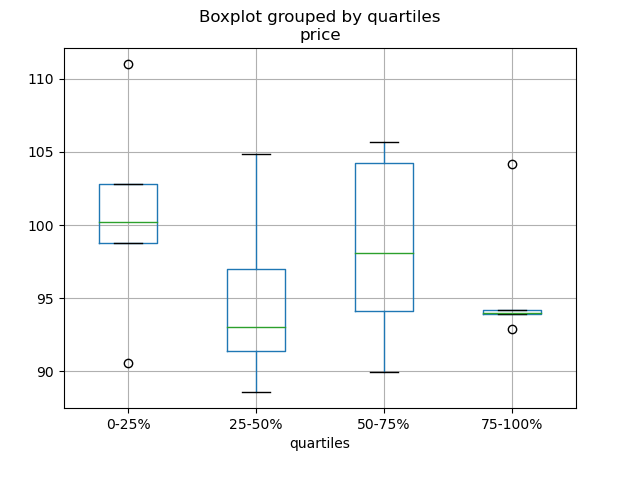
用 Pandas、Vincent、xlsxwriter 生成 Excel 文件里的嵌入可视图

为分层变量的每个四分位数绘制箱型图

In [186]: df = pd.DataFrame(
   .....:     {'stratifying_var': np.random.uniform(0, 100, 20),
   .....:      'price': np.random.normal(100, 5, 20)})
   .....: 
In [187]: df['quartiles'] = pd.qcut(
   .....:     df['stratifying_var'],
   .....:     4,
   .....:     labels=['0-25%', '25-50%', '50-75%', '75-100%'])
   .....: 
In [188]: df.boxplot(column='price', by='quartiles')
Out[188]: <matplotlib.axes._subplots.AxesSubplot at 0x7efff077f910>

../_images/quartile_boxplot.png

数据输入输出

SQL 与 HDF5 性能对比

CSV

CSV文档

read_csv 函数实战

把 DataFrame 追加到 CSV 文件

分块读取 CSV

分块读取指定的行

只读取 DataFrame 的前几列

读取不是 gzip 或 bz2 压缩（read_csv 可识别的内置压缩格式）的文件。本例在介绍如何读取 WinZip 压缩文件的同时，还介绍了在环境管理器里打开文件，并读取内容的通用操作方式。详见本链接

推断文件数据类型

处理出错数据

处理出错数据 II

用 Unix 时间戳读取 CSV，并转为本地时区

写入多行索引 CSV 时，不写入重复值

从多个文件读取数据，创建单个 DataFrame

最好的方式是先一个个读取单个文件，然后再把每个文件的内容存成列表，再用 pd.concat() 组合成一个 DataFrame:

In [189]: for i in range(3):
   .....:     data = pd.DataFrame(np.random.randn(10, 4))
   .....:     data.to_csv('file_{}.csv'.format(i))
   .....: 
In [190]: files = ['file_0.csv', 'file_1.csv', 'file_2.csv']
In [191]: result = pd.concat([pd.read_csv(f) for f in files], ignore_index=True)

还可以用同样的方法读取所有匹配同一模式的文件，下面这个例子使用的是glob：

In [192]: import glob
In [193]: import os
In [194]: files = glob.glob('file_*.csv')
In [195]: result = pd.concat([pd.read_csv(f) for f in files], ignore_index=True)

最后，这种方式也适用于 io 文档介绍的其它 pd.read_* 函数。

解析多列里的日期组件

用一种格式解析多列的日期组件，速度更快。

In [196]: i = pd.date_range('20000101', periods=10000)
In [197]: df = pd.DataFrame({'year': i.year, 'month': i.month, 'day': i.day})
In [198]: df.head()
Out[198]: 
   year  month  day
0  2000      1    1
1  2000      1    2
2  2000      1    3
3  2000      1    4
4  2000      1    5
In [199]: %timeit pd.to_datetime(df.year * 10000 + df.month * 100 + df.day, format='%Y%m%d')
   .....: ds = df.apply(lambda x: "%04d%02d%02d" % (x['year'],
   .....:                                           x['month'], x['day']), axis=1)
   .....: ds.head()
   .....: %timeit pd.to_datetime(ds)
   .....: 
10.6 ms +- 698 us per loop (mean +- std. dev. of 7 runs, 100 loops each)
3.21 ms +- 36.4 us per loop (mean +- std. dev. of 7 runs, 100 loops each)

跳过标题与数据之间的行

In [200]: data = """;;;;
   .....:  ;;;;
   .....:  ;;;;
   .....:  ;;;;
   .....:  ;;;;
   .....:  ;;;;
   .....: ;;;;
   .....:  ;;;;
   .....:  ;;;;
   .....: ;;;;
   .....: date;Param1;Param2;Param4;Param5
   .....:     ;m²;°C;m²;m
   .....: ;;;;
   .....: 01.01.1990 00:00;1;1;2;3
   .....: 01.01.1990 01:00;5;3;4;5
   .....: 01.01.1990 02:00;9;5;6;7
   .....: 01.01.1990 03:00;13;7;8;9
   .....: 01.01.1990 04:00;17;9;10;11
   .....: 01.01.1990 05:00;21;11;12;13
   .....: """
   .....:

选项 1：显式跳过行

In [201]: from io import StringIO
In [202]: pd.read_csv(StringIO(data), sep=';', skiprows=[11, 12],
   .....:             index_col=0, parse_dates=True, header=10)
   .....: 
Out[202]: 
                     Param1  Param2  Param4  Param5
date                                               
1990-01-01 00:00:00       1       1       2       3
1990-01-01 01:00:00       5       3       4       5
1990-01-01 02:00:00       9       5       6       7
1990-01-01 03:00:00      13       7       8       9
1990-01-01 04:00:00      17       9      10      11
1990-01-01 05:00:00      21      11      12      13

选项 2：读取列名，然后再读取数据

In [203]: pd.read_csv(StringIO(data), sep=';', header=10, nrows=10).columns
Out[203]: Index(['date', 'Param1', 'Param2', 'Param4', 'Param5'], dtype='object')
In [204]: columns = pd.read_csv(StringIO(data), sep=';', header=10, nrows=10).columns
In [205]: pd.read_csv(StringIO(data), sep=';', index_col=0,
   .....:             header=12, parse_dates=True, names=columns)
   .....: 
Out[205]: 
                     Param1  Param2  Param4  Param5
date                                               
1990-01-01 00:00:00       1       1       2       3
1990-01-01 01:00:00       5       3       4       5
1990-01-01 02:00:00       9       5       6       7
1990-01-01 03:00:00      13       7       8       9
1990-01-01 04:00:00      17       9      10      11
1990-01-01 05:00:00      21      11      12      13

SQL

SQL 文档

用 SQL 读取数据库

Excel

Excel 文档

读取文件式句柄

用 XlsxWriter 修改输出格式

HTML

从不能处理默认请求 header 的服务器读取 HTML 表格

HDFStore

HDFStores文档

按块对大规模数据存储去重的本质是递归还原操作。这里介绍了一个函数，可以从 CSV 文件里按块提取数据，解析日期后，再按块存储。

把属性存至分组节点

In [206]: df = pd.DataFrame(np.random.randn(8, 3))
In [207]: store = pd.HDFStore('test.h5')
In [208]: store.put('df', df)
# 用 pickle 存储任意 Python 对象
In [209]: store.get_storer('df').attrs.my_attribute = {'A': 10}
In [210]: store.get_storer('df').attrs.my_attribute
Out[210]: {'A': 10}

二进制文件

读取 C 结构体数组组成的二进制文件，Pandas 支持 NumPy 记录数组。比如说，名为 main.c 的文件包含下列 C 代码，并在 64 位机器上用 gcc main.c -std=gnu99 进行编译。

#include <stdio.h>
#include <stdint.h>
typedef struct _Data
{
    int32_t count;
    double avg;
    float scale;
} Data;
int main(int argc, const char *argv[])
{
    size_t n = 10;
    Data d[n];
    for (int i = 0; i < n; ++i)
    {
        d[i].count = i;
        d[i].avg = i + 1.0;
        d[i].scale = (float) i + 2.0f;
    }
    FILE *file = fopen("binary.dat", "wb");
    fwrite(&d, sizeof(Data), n, file);
    fclose(file);
    return 0;
}

下列 Python 代码读取二进制二建 binary.dat，并将之存为 pandas DataFrame，每个结构体的元素对应 DataFrame 里的列：

names = 'count', 'avg', 'scale'
# 注意：因为结构体填充，位移量比类型尺寸大
offsets = 0, 8, 16
formats = 'i4', 'f8', 'f4'
dt = np.dtype({'names': names, 'offsets': offsets, 'formats': formats},
              align=True)
df = pd.DataFrame(np.fromfile('binary.dat', dt))

::: tip 注意

不同机器上创建的文件因其架构不同，结构化元素的位移量也不同，原生二进制格式文件不能跨平台使用，因此不建议作为通用数据存储格式。建议用 Pandas IO 功能支持的 HDF5 或 msgpack 文件。

:::

计算

基于采样的时间序列数值整合

时间差

时间差文档。

使用时间差

In [218]: import datetime
In [219]: s = pd.Series(pd.date_range('2012-1-1', periods=3, freq='D'))
In [220]: s - s.max()
Out[220]: 
0   -2 days
1   -1 days
2    0 days
dtype: timedelta64[ns]
In [221]: s.max() - s
Out[221]: 
0   2 days
1   1 days
2   0 days
dtype: timedelta64[ns]
In [222]: s - datetime.datetime(2011, 1, 1, 3, 5)
Out[222]: 
0   364 days 20:55:00
1   365 days 20:55:00
2   366 days 20:55:00
dtype: timedelta64[ns]
In [223]: s + datetime.timedelta(minutes=5)
Out[223]: 
0   2012-01-01 00:05:00
1   2012-01-02 00:05:00
2   2012-01-03 00:05:00
dtype: datetime64[ns]
In [224]: datetime.datetime(2011, 1, 1, 3, 5) - s
Out[224]: 
0   -365 days +03:05:00
1   -366 days +03:05:00
2   -367 days +03:05:00
dtype: timedelta64[ns]
In [225]: datetime.timedelta(minutes=5) + s
Out[225]: 
0   2012-01-01 00:05:00
1   2012-01-02 00:05:00
2   2012-01-03 00:05:00
dtype: datetime64[ns]

日期加减

In [226]: deltas = pd.Series([datetime.timedelta(days=i) for i in range(3)])
In [227]: df = pd.DataFrame({'A': s, 'B': deltas})
In [228]: df
Out[228]: 
           A      B
0 2012-01-01 0 days
1 2012-01-02 1 days
2 2012-01-03 2 days
In [229]: df['New Dates'] = df['A'] + df['B']
In [230]: df['Delta'] = df['A'] - df['New Dates']
In [231]: df
Out[231]: 
           A      B  New Dates   Delta
0 2012-01-01 0 days 2012-01-01  0 days
1 2012-01-02 1 days 2012-01-03 -1 days
2 2012-01-03 2 days 2012-01-05 -2 days
In [232]: df.dtypes
Out[232]: 
A             datetime64[ns]
B            timedelta64[ns]
New Dates     datetime64[ns]
Delta        timedelta64[ns]
dtype: object

其它示例

与 datetime 类似，用 np.nan 可以把值设为 NaT。

In [233]: y = s - s.shift()
In [234]: y
Out[234]: 
0      NaT
1   1 days
2   1 days
dtype: timedelta64[ns]
In [235]: y[1] = np.nan
In [236]: y
Out[236]: 
0      NaT
1      NaT
2   1 days
dtype: timedelta64[ns]

轴别名

设置全局轴别名，可以定义以下两个函数：

In [237]: def set_axis_alias(cls, axis, alias):
   .....:     if axis not in cls._AXIS_NUMBERS:
   .....:         raise Exception("invalid axis [%s] for alias [%s]" % (axis, alias))
   .....:     cls._AXIS_ALIASES[alias] = axis
   .....: 
In [238]: def clear_axis_alias(cls, axis, alias):
   .....:     if axis not in cls._AXIS_NUMBERS:
   .....:         raise Exception("invalid axis [%s] for alias [%s]" % (axis, alias))
   .....:     cls._AXIS_ALIASES.pop(alias, None)
   .....: 
In [239]: set_axis_alias(pd.DataFrame, 'columns', 'myaxis2')
In [240]: df2 = pd.DataFrame(np.random.randn(3, 2), columns=['c1', 'c2'],
   .....:                    index=['i1', 'i2', 'i3'])
   .....: 
In [241]: df2.sum(axis='myaxis2')
Out[241]: 
i1   -0.461013
i2    2.040016
i3    0.904681
dtype: float64
In [242]: clear_axis_alias(pd.DataFrame, 'columns', 'myaxis2')

创建示例数据

类似 R 的 expand.grid() 函数，用不同类型的值组生成 DataFrame，需要创建键是列名，值是数据值列表的字典：

In [243]: def expand_grid(data_dict):
   .....:     rows = itertools.product(*data_dict.values())
   .....:     return pd.DataFrame.from_records(rows, columns=data_dict.keys())
   .....: 
In [244]: df = expand_grid({'height': [60, 70],
   .....:                   'weight': [100, 140, 180],
   .....:                   'sex': ['Male', 'Female']})
   .....: 
In [245]: df
Out[245]: 
    height  weight     sex
0       60     100    Male
1       60     100  Female
2       60     140    Male
3       60     140  Female
4       60     180    Male
5       60     180  Female
6       70     100    Male
7       70     100  Female
8       70     140    Male
9       70     140  Female
10      70     180    Male
11      70     180  Female

烹饪指南

烹饪指南

惯用语

if-then…

切割

设置条件

选择

DataFrames

生成新列

多层索引

运算

切片

排序

层级

缺失数据

替换

分组

扩展数据

分割

透视表

Apply 函数

时间序列

重采样

合并

可视化

数据输入输出

CSV

从多个文件读取数据，创建单个 DataFrame

解析多列里的日期组件

跳过标题与数据之间的行

选项 1：显式跳过行

选项 2：读取列名，然后再读取数据

SQL

Excel

HTML

HDFStore

二进制文件

计算

相关性

时间差

轴别名

创建示例数据