插入排序 | Insertion Sort
插入排序将数列划分为“已排序的”和“未排序的”两部分,每次从“未排序的”元素中选择一个插入到“已排序的”元素中的正确位置。
for (int i = 1; i < N; i++) {int temp = a[i];for (int j = i; j > 0 && a[j-1] > temp; j--)a[j] = a[j-1]; //overwritea[j] = temp;}
插入排序的最坏情况时间复杂度和平均情况时间复杂度都为 ,但其在数列几乎有序时效率很高,在数列是完全有序的情况下时间复杂度是  的。一般地,复杂度精确的为,为序列中逆序对的数目。<br />**逆序对的定义:**的一对。
 个互异数的平均逆序数是
 ,完全反序是
 。
。- 通过交换相邻元素来进行排序的任何算法平均需要
 时间。
时间。
希尔排序 | Shell Sort
希尔排序可以看做插入排序的一般化,定义增量序列 ,在用增量
,在用增量 排序后,对所有
 ,均有
,均有 ,称为
,称为 。其重要的性质也是算法的基础是,
 后的序列将保持
 排序的特性不改变。
对于增量序列的选取直接影响算法的复杂度,我们以 为例。
为例。
int i, j, increment, temp;for (increment = N / 2; increment > 0; increment /= 2){for (i = increment; i < N; i++){temp = a[i];for (j = i; j >= increment; j -= increment){if( temp < a[j - increment]) a[j] = a[j - increment];else break;}a[j] = temp;}}
Hibbard增量序列
- Hibbard增量序列的希尔排序上界为
 ,平均运行时间为
 。
。 - Hibbard序列:

Sedgewick增量序列(已知最好的序列)
- 上界为
 ,平均为
,平均为 。
。 - Sedgewick序列:

堆排序 | Heap Sort
之前学堆的时候自己写过一个堆排序,但是空间的需求是双倍,因为要重新建堆
void Heapsort( ElementType A[ ], int N ) {int i;for ( i = N / 2; i >= 0; i - - ) /* BuildHeap */PercDown( A, i, N );for ( i = N - 1; i > 0; i - - ) {Swap( &A[ 0 ], &A[ i ] ); /* DeleteMax */PercDown( A, 0, i );}
改删除为放置于队尾,同时堆的大小减小(即`PercDown()`的第三个参数),这样可在原数组的基础上进行堆排序,空间需求仍为。
归并排序 | Merge Sort
经典的分治算法例子,我们看这个图会很清楚: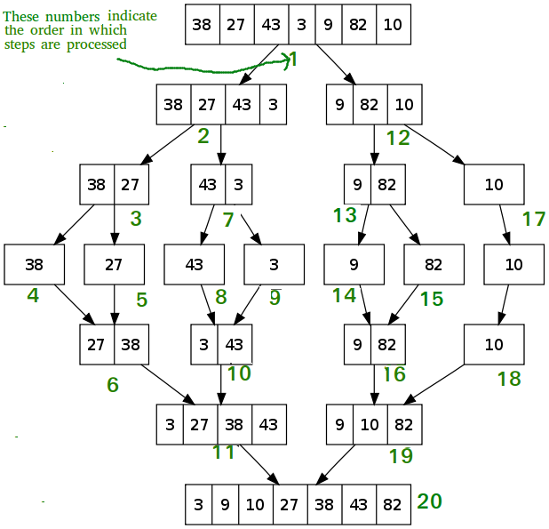
快速排序 | Quick Sort(undone)
桶排序、基数排序 | Bucket&Radix Sort(undone)
算法稳定性
稳定性是指具有相同值的元素在排序过程中的相对位置是否变化,若变化,不稳定,反之则稳定
- 插入排序:稳定,因为一个个
- 希尔排序:不稳定,因为交换
- 快速排序:不稳定,因为排序后交换
- 堆排序:不稳定,直接拉到最上面交换
- 归并排序:稳定,指针一个个移动
- 基数排序:稳定

若有收获,就点个赞吧
0 人点赞
