时间
as.Date(‘2017-02-16’,format = ) format是指定前面时间的格式
%m :数字月份
%b:jan
%B:july
%Y:四位数年份
%y:两位数年份
%a Mon
%A Monday
> as.Date('2/16/2017',format = '%m/%d/%Y')[1] "2017-02-16"> as.Date('March 10, 1993', format = '%B %d, %Y')[1] NA> as.Date('10Mar93','%d%b%y') #不存在的日期返回NA[1] NA> as.Date(100, origin = '2017-02-16') #指定开始时间,后面加天数[1] "2017-05-27"
ISOdate
> ISOdate(1993,3,10,16,14,20)[1] "1993-03-10 16:14:20 GMT"
POSIX
> dts <- c('2005-10-21 18:24:24', "2017-02-16 19:20:20")> as.POSIXlt(dts)[1] "2005-10-21 18:24:24 CST" "2017-02-16 19:20:20 CST"
strptime() and strftime()
> time <- strptime('04/3/2016:16:18:34', format = '%d/%m/%Y:%H:%M:%S');time[1] "2016-03-04 16:18:34 CST"> strftime(time, 'Now is %H:%M on %Y %m %d')[1] "Now is 16:18 on 2016 03 04"
julian 计算天数
> julian(as.Date('2017-02-16'), origin = as.Date('2016-02-19'))[1] 363attr(,"origin")[1] "2016-02-19"> julian(as.Date('2017-02-16')) #默认是1970-01-01[1] 17213attr(,"origin")[1] "1970-01-01"
difftime 计算时间差,mean计算中间时间,dateline生成间隔时间
> difftime(as.Date('2017-02-16'),as.Date('2016-02-19'),units = 'weeks')Time difference of 51.85714 weeks> difftime(as.Date(now()),as.Date("1987-07-13"),units = "day")Time difference of 12241 days> difftime(as.Date("2067-07-13"),as.Date("1987-07-13"),units = "day")Time difference of 29220 days> mean(c(as.Date('2017-02-16'),as.Date('2016-02-19')))[1] "2016-08-18"> dateline <- seq(as.Date('2016-02-10'), by = '2 weeks', length.out = 10);dateline[1] "2016-02-10" "2016-02-24" "2016-03-09" "2016-03-23" "2016-04-06"[6] "2016-04-20" "2016-05-04" "2016-05-18" "2016-06-01" "2016-06-15"> dateline <- seq(as.Date('2016-02-10'), by = '2 days', length.out = 10);dateline[1] "2016-02-10" "2016-02-12" "2016-02-14" "2016-02-16" "2016-02-18"[6] "2016-02-20" "2016-02-22" "2016-02-24" "2016-02-26" "2016-02-28"
用stringi处理时间
> library(stringi)> (my_newtime <- stri_datetime_add(as.Date('2017-02-16'), value = 10, units = 'days'))[1] "2017-02-26 08:00:00 CST"> stri_datetime_create(2014,4,20)[1] "2014-04-20 12:00:00 CST"> stri_datetime_parse(c('2015-02-27','2015-02-29'), 'yyyy-MM-dd')[1] "2015-02-27 20:01:51 CST" NA> stri_datetime_parse(c('2015-02-27','2015-02-29'), 'yyyy-MM-dd', lenient = TRUE) #lenient = TRUE不存在该时间时,自动往后生成正确的时间[1] "2015-02-27 20:00:17 CST" "2015-03-01 20:00:17 CST"> stri_datetime_parse('DEC-29','LLL-dd') #这个函数现在不能识别了MMM 和LLL[1] NA> stri_datetime_parse('02-20','MM-dd')[1] "2021-02-20 20:00:18 CST"> stri_datetime_parse('DEC-05','MMM-dd')[1] NA> stri_datetime_format(stri_datetime_now(), 'datetime_relative_medium')[1] "今天 下午8:00:20"
Lubridate包
ymd(a)直接将a转换年月日格式
myd(a)直接将a转换月年日格式
ymd_hms 加了时分秒
month,day ,year可以直接提取其中的月日年,label是标签,abbr是简称
mday返回在月份的顺序,wday返回在星期中的顺序
now()返回现在的时间
make_datetime()返回最初的原时间1970-1-1
make_date(year,month,day)生成时间
round_date()生成近似时间,不是四舍五入,是看哪个比较近
> library(lubridate)> ymd('020217')[1] "2002-02-17"> mdy('06182016')[1] "2016-06-18"> x <- c('2009s01s01','2009-01-02','2009 01 03','2009,1,4','09.1.1','leopard 09 12 09', '!!09 ## 12 $$ 12')> x_time <- ymd(x);x_time[1] "2009-01-01" "2009-01-02" "2009-01-03" "2009-01-04" "2009-01-01"[6] "2009-12-09" "2009-12-12"> ymd_hms('2017 02 19 14 23 23')[1] "2017-02-19 14:23:23 UTC"> month(x_time, label = T, abbr = F)[1] 一月 一月 一月 一月 一月 十二月 十二月12 Levels: 一月 < 二月 < 三月 < 四月 < 五月 < 六月 < 七月 < ... < 十二月> month(x_time, label = T, abbr = T)[1] 1 1 1 1 1 12 12Levels: 1 < 2 < 3 < 4 < 5 < 6 < 7 < 8 < 9 < 10 < 11 < 12> month(x_time, label = F)[1] 1 1 1 1 1 12 12> day(x_time)[1] 1 2 3 4 1 9 12> mday(x_time)[1] 1 2 3 4 1 9 12> wday(x_time)[1] 5 6 7 1 5 4 7> new_date <- now();new_date[1] "2021-01-16 20:32:19 CST"> month(new_date) <- 12> new_date[1] "2021-12-16 20:32:19 CST"> dates <- make_date(year = 2010:2016,month = 1:3,day = 1:5)> dates[1] "2010-01-01" "2011-02-02" "2012-03-03" "2013-01-04" "2014-02-05"[6] "2015-03-01" "2016-01-02"> make_datetime()[1] "1970-01-01 UTC"> x_time <- as.POSIXlt('2009-08-03 12:01:59');x_time> round_date(x_time, unit = 'minutes')[1] "2009-08-03 12:02:00 CST"> round_date(x_time, unit = 'day')[1] "2009-08-04 CST"> round_date(x_time, unit = 'halfyear')[1] "2009-07-01 CST"> time_t <- c('2017-02','201609','2017/5')
补全日期
> time_t <- c('2017-02','201609','2017/5')
> ymd(time_t)
[1] NA NA NA
Warning message:
All formats failed to parse. No formats found.
> ymd(time_t,truncated = 1) # 补全日期,1和2没有区别
[1] "2017-02-01" "2016-09-01" "2017-05-01"
> ymd(time_t,truncated = 2)
[1] "2017-02-01" "2016-09-01" "2017-05-01"
计算时间差 difftime更好用
> time_tt <- ymd('1900,01,01','1999,12,31')
> int <- interval(start = ymd('1900,01,01'),end = ymd('1999,12,31'));int
[1] 1900-01-01 UTC--1999-12-31 UTC
> time_length(int,unit = 'day')
[1] 36523
> time_length(int,unit = 'year')
[1] 99.99726
时间加法
> x <- as.POSIXlt('2017-02-03');x
[1] "2017-02-03 CST"
> x + days(10) + hours(12) + minutes(30)
[1] "2017-02-13 12:30:00 CST"
时间序列
ts()生成时间序列
> #ts()生成时间序列
> ts(1:10, frequency = 4, start = c(1999, 2),end = c(2001,3)) #4个月为间隔
     Qtr1 Qtr2 Qtr3 Qtr4
1999         1    2    3
2000    4    5    6    7
2001    8    9   10
> ts(1:10, frequency = 4, start = c(1999, 5),end = c(2001,3)) #4个月为间隔,注意5
     Qtr1 Qtr2 Qtr3 Qtr4
2000    1    2    3    4
2001    5    6    7
> ts(1:10, frequency = 12, start = c(1999, 4),end = c(2001,3))#12个月为间隔
     Jan Feb Mar Apr May Jun Jul Aug Sep Oct Nov Dec
1999               1   2   3   4   5   6   7   8   9
2000  10   1   2   3   4   5   6   7   8   9  10   1
2001   2   3   4
> ts(1:10, frequency = 12, start = c(1999, 13),end = c(2001,3))#12个月为间隔 注意13
     Jan Feb Mar Apr May Jun Jul Aug Sep Oct Nov Dec
2000   1   2   3   4   5   6   7   8   9  10   1   2
2001   3   4   5

> ts(1:10, frequency = 12, start = c(1999, 13))
     Jan Feb Mar Apr May Jun Jul Aug Sep Oct
2000   1   2   3   4   5   6   7   8   9  10
实例
- value 按照start开始的时间到end结束的时间,频率是每天,生成一个数,数有sample随机生成
- date 生成时间序列
- df 将时间和数值组成数据框
> value <- ts(data = sample(0:300,366,replace = TRUE),start = as.Date('2016-01-01'), frequency = 1,end = as.Date('2016-12-31'))
> date <- seq(from = as.Date('2016-01-01'),by = 1, length.out = 366)
> df <- data.frame(value = value, time = date)
> plot(ts(cumsum(1+round(rnorm(100),2)), start = c(1954,7), frequency = 12)) #cumsum累积和,后面一个数为前面俩个数的和
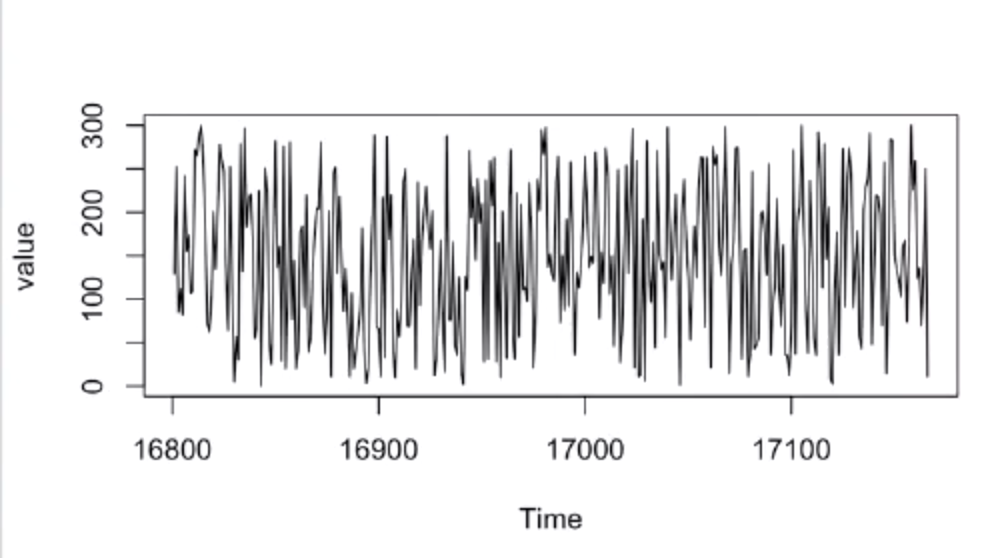
> plot(value)
xts包
> library(xts)
> value <- sample(0:100, 365, replace = T)
> times <- seq(from = as.Date('2017-01-01'), by = 1, length = 365)
> myts <- xts(value, times)
> head(myts)
           [,1]
2017-01-01   64
2017-01-02   45
2017-01-03   22
2017-01-04   65
2017-01-05    6
2017-01-06    9
> window(myts, start = as.Date('2017-01-10'), end = as.Date('2017-01-15')) #取值
           [,1]
2017-01-10   42
2017-01-11   14
2017-01-12   90
2017-01-13   12
2017-01-14   18
2017-01-15   21
> window(myts, start = as.Date('2017-01-1'), end = as.Date('2017-01-6')) <- 1:6 #赋值
> head(myts)
           [,1]
2017-01-01    1
2017-01-02    2
2017-01-03    3
2017-01-04    4
2017-01-05    5
2017-01-06    6
lag 是指将前后的值赋值给后面,diff是指减去前一个时间
> myts <- xts(value, times)
> head(myts)
           [,1]
2017-01-01   64
2017-01-02   45
2017-01-03   22
2017-01-04   65
2017-01-05    6
2017-01-06    9
> head(lag(myts))
           [,1]
2017-01-01   NA
2017-01-02   64
2017-01-03   45
2017-01-04   22
2017-01-05   65
2017-01-06    6
> head(diff(myts))
           [,1]
2017-01-01   NA
2017-01-02  -19
2017-01-03  -23
2017-01-04   43
2017-01-05  -59
2017-01-06    3
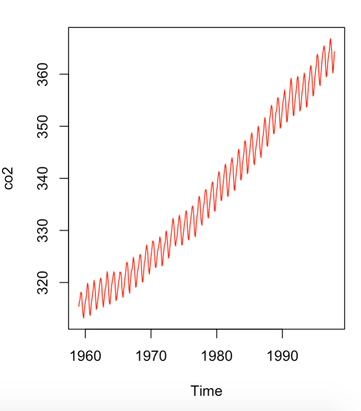
实例:co2数据集
> data("co2") #co2数据集
> class(co2)
[1] "ts"
> head(co2)
[1] 315.42 316.31 316.50 317.56 318.13 318.00
> length(co2)
[1] 468
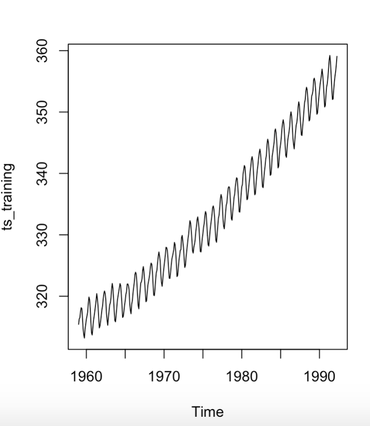
> training <- co2[1:400]
> ts_training <- ts(training, start = start(co2), frequency = frequency(co2))
> plot(ts_training)
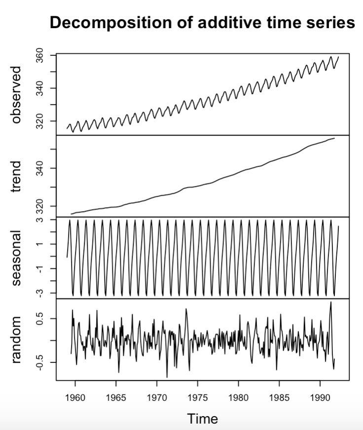
> de_co2 <- decompose(ts_training)
> plot(de_co2)
> library(tseries)
> training <- co2[1:400]
> ts_training <- ts(training, start = start(co2), frequency = frequency(co2))
> kpss.test(ts_training)
KPSS Test for Level Stationarity
data: ts_training
KPSS Level = 6.6342, Truncation lag parameter = 5, p-value = 0.01
Warning message:
In kpss.test(ts_training) : p-value smaller than printed p-value
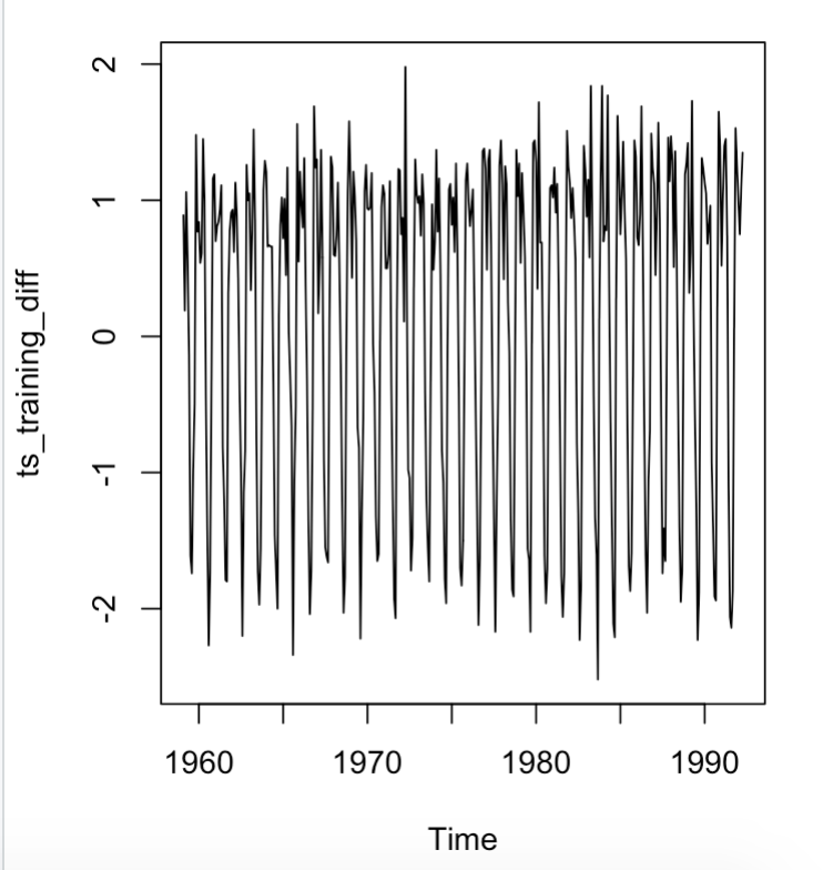
> ts_training_diff <- diff(ts_training)
> kpss.test(ts_training_diff)
KPSS Test for Level Stationarity
data: ts_training_diff
KPSS Level = 0.023192, Truncation lag parameter = 5, p-value = 0.1
Warning message:
In kpss.test(ts_training_diff) : p-value greater than printed p-value
> plot(ts_training_diff)
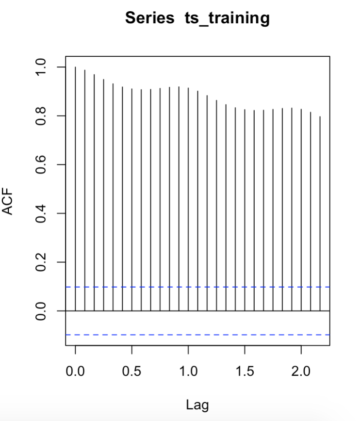
acf(ts_training)
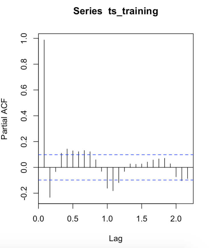
pacf(ts_training)


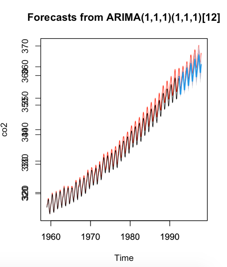
Arima建模,forecast预测
> library(forecast)
# ARIMA(P,D,Q)
> co2_fit <- Arima(ts_training, order = c(1,1,1),
+                  seasonal = list(order = c(1,1,1), period = 12))
> co2_fore <- forecast(co2_fit, 68)
> plot(co2, col = 'red')
> par(new = TRUE)
> par(new = TRUE)
> plot(co2_fore)

若有收获,就点个赞吧
0 人点赞
