计算激活函数
Sigmoid和ReLU
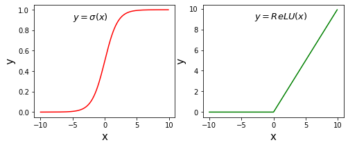
使用ndarray数组可以很方便的构建数学函数,并利用其底层的矢量计算能力快速实现计算。下面以神经网络中比较常用激活函数Sigmoid和ReLU为例,介绍代码实现过程。
- 计算Sigmoid激活函数

- 计算ReLU激活函数

使用Numpy计算激活函数Sigmoid和ReLU的值,使用matplotlib画出图形,代码如下所示。
# ReLU和Sigmoid激活函数示意图import numpy as npimport matplotlib.pyplot as pltimport matplotlib.patches as patches%matplotlib inline#设置图片大小plt.figure(figsize=(8, 3))# x是1维数组,数组大小是从-10. 到10.的实数,每隔0.1取一个点x = np.arange(-10, 10, 0.1)# 计算 Sigmoid函数s = 1.0 / (1 + np.exp(- x))# 计算ReLU函数y = np.clip(x, a_min = 0., a_max = None)########################################################## 以下部分为画图程序# 设置两个子图窗口,将Sigmoid的函数图像画在左边f = plt.subplot(121)# 画出函数曲线plt.plot(x, s, color='r')# 添加文字说明plt.text(-5., 0.9, r'$y=\sigma(x)$', fontsize=13)# 设置坐标轴格式currentAxis=plt.gca()currentAxis.xaxis.set_label_text('x', fontsize=15)currentAxis.yaxis.set_label_text('y', fontsize=15)# 将ReLU的函数图像画在右边f = plt.subplot(122)# 画出函数曲线plt.plot(x, y, color='g')# 添加文字说明plt.text(-3.0, 9, r'$y=ReLU(x)$', fontsize=13)# 设置坐标轴格式currentAxis=plt.gca()currentAxis.xaxis.set_label_text('x', fontsize=15)currentAxis.yaxis.set_label_text('y', fontsize=15)plt.show()
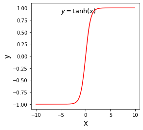
tanh
tanh 的函数定义如下:
import numpy as npimport matplotlib.pyplot as pltimport matplotlib.patches as patches%matplotlib inline#设置图片大小plt.figure(figsize=(6, 4))# x是1维数组,数组大小是从-10. 到10.的实数,每隔0.1取一个点x = np.arange(-10, 10, 0.1)# 计算 tanh 函数s = (np.exp(x) - np.exp(-x)) / (np.exp(x) + np.exp(-x))# 画出函数曲线plt.plot(x, s, color='r')# 添加文字说明plt.text(-5., 0.9, r'$y=\tanh(x)$', fontsize=13)# 设置坐标轴格式currentAxis=plt.gca()currentAxis.xaxis.set_label_text('x', fontsize=15)currentAxis.yaxis.set_label_text('y', fontsize=15)plt.show()
使用numpy作数字图像处理
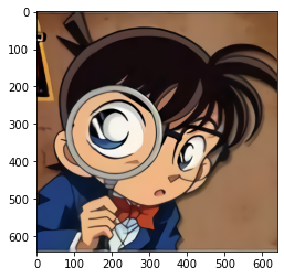
图像是由像素点构成的矩阵,其数值可以用ndarray来表示。将上述介绍的操作用在图像数据对应的ndarray上,可以很轻松的实现图片的翻转、裁剪和亮度调整,具体代码和效果如下所示。
# 导入需要的包import numpy as npimport matplotlib.pyplot as pltfrom PIL import Image# 读入图片image = Image.open('./work/logo.png')image = np.array(image)
查看数据形状,其形状是[H, W, 3],其中H代表高度, W是宽度,3代表RGB三个通道
>>> image.shape(640, 640, 3)
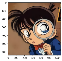
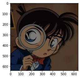
查看原始图像:
plt.imshow(image)
输出:
<matplotlib.image.AxesImage at 0x1fb6072b788>
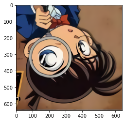
翻转
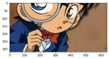
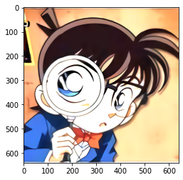
垂直方向翻转
垂直翻转,其实就是将图像的第一行跟最后一行置换,第(n-1)行跟第(2)行置换…:
image2 = image[::-1, :, :]plt.imshow(image2)
水平方向翻转
跟垂直方向翻转原理一致,在第二个维度做处理即可:
image3 = image[:, ::-1, :]plt.imshow(image3)
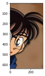
剪裁
有了刚才翻转的基础,其实剪裁很好理解,就是在某一个维度上设置起始位置和终止位置即可:
# 高度方向裁剪H, W = image.shape[0], image.shape[1]# 注意此处用整除,H_start必须为整数image4 = image[H//2:H, :, :]plt.imshow(image4)
# 宽度方向裁剪H, W = image.shape[0], image.shape[1]image5 = image[:, W//2:W, :]plt.imshow(image5)
# 两个方向同时裁剪image5 = image[H//2:H, W//2:W, :]plt.imshow(image5)
调整亮度
将每个像素点(包含RGB三色信息)同时乘以同一个标量,即可以改变图像的亮度,注意:RGB像素值最高到255。
减少亮度**
image6 = image * 0.5plt.imshow(image6.astype('uint8'))
增加亮度
image7 = image * 2.0# 由于图片的RGB像素值必须在0-255之间,此处使用np.clip进行数值裁剪image7 = np.clip(image7, a_min=None, a_max=255.)plt.imshow(image7.astype('uint8'))
拉伸及压缩图片
拉伸及压缩图片有很多策略,比如以下策略:
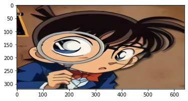
高度方向每隔一行取像素点**
image8 = image[::2, :, :]plt.imshow(image8)
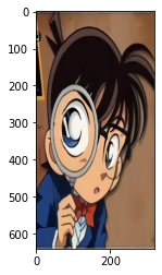
宽度方向每隔一列取像素点
image9 = image[:, ::2, :]plt.imshow(image9)
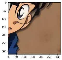
间隔行列采样
间隔行列采样,图像尺寸会减半,清晰度变差
image10 = image[::2, ::2, :]plt.imshow(image10)

保存图像至文件
同样通过save保存即可:
outputImage = Image.fromarray(image3)outputImage.save('output.jpg')

若有收获,就点个赞吧
0 人点赞
