开发环境：Google Colab

卷积 GAN - Celeba 生成人脸图像

14_gan_cnn_celeba.ipynb

• 挂载驱动器以访问 google drive 中的文件

  # mount Drive to access data files
  from google.colab import drive
  drive.mount('./mount')

• 导入包 ```python import torch import torch.nn as nn from torch.utils.data import Dataset

import h5py import pandas, numpy, random import matplotlib.pyplot as plt

- 标准的CUDA检查和设置步骤
```python
# 检查CUDA是否可用，如果可用，则设置默认的rensor类型为cuda
# 使用CUDA需要在上方工具栏“代码执行程序-更改运行时类型-硬件加速器”改为GPU
if torch.cuda.is_available():
  torch.set_default_tensor_type(torch.cuda.FloatTensor)
  print("using cuda:", torch.cuda.get_device_name(0))
  pass
device = torch.device("cuda" if torch.cuda.is_available() else "cpu")
device

辅助函数

# 生成随机数据
def generate_random_image(size):
    random_data = torch.rand(size)  # 生成的数据符合0-1区间内的均匀分布
    return random_data
def generate_random_seed(size):
    random_data = torch.randn(size) # 生成的数据符合均值为0，方差为1的正态分布
    return random_data

# 将三维张量转换为一维张量（eg. 将大小为(218, 178, 3)的三维图像张量重塑成一个长度为218*178*3的一维张量）
# modified from https://github.com/pytorch/vision/issues/720
class View(nn.Module):
  def __init__(self, shape):
    super().__init__()
    self.shape = shape,
  def forward(self, x):
    return x.view(*self.shape)

# 将一个给定的numpy图像中裁剪为指定的长和宽，裁剪的区域位于输入图像的正中央
def crop_centre(img, new_width, new_height):
  height, width, _ = img.shape
  startx = width // 2 - new_width // 2    # 注意使用整数除法//
  starty = height // 2 - new_height // 2
  return img[ starty: starty + new_height, startx: startx + new_width, :]

数据集类

# 数据集类
class CelebADataset(Dataset):
  def __init__(self, file):
    self.file_object = h5py.File(file, 'r')
    self.dataset = self.file_object['img_align_celeba']
    pass
  def __len__(self):
    return len(self.dataset)
  def __getitem__(self, index):
    if(index >= len(self.dataset)):
      raise IndexError()
    img = numpy.array(self.dataset[str(index)+'.jpg'])
    # 将图像裁剪为128*128大小的正方形图像
    img = crop_centre(img, 128, 128)
    return torch.cuda.FloatTensor(img).permute(2, 0, 1).view(1, 3, 128, 128) / 255.0  # 使得结果范围在0-1
    # 最终返回一个四维张量的形式：（批次大小，通道数，高度，宽度）
    # 原本numpy数组的形式为（高度，宽度，通道数3）的三维张量，因此先用permute(2, 0, 1)将numpy数组重新排序为（通道数3，高度，宽度）
    # 再使用view(1, 3, 128, 128)增加一个额外的维度，代表批量大小，这里为1
  def plot_image(self, index):
    if(index >= len(self.dataset)):
      raise IndexError()
    img = numpy.array(self.dataset[str(index)+'.jpg'])
    # 将图像裁剪为128*128大小的正方形图像
    img = crop_centre(img, 128, 128)
    plt.imshow(img, interpolation='nearest')
    pass
  pass

# 创建数据集对象
celeba_dataset = CelebADataset('mount/My Drive/Colab Notebooks/pytorch_gan/celeba_data/celeba_aligned_small.h5py')

# 检查数据集中的图像 & 检查图像是否正确被裁减
celeba_dataset.plot_image(43) # 索引范围是0-19999

鉴别器网络

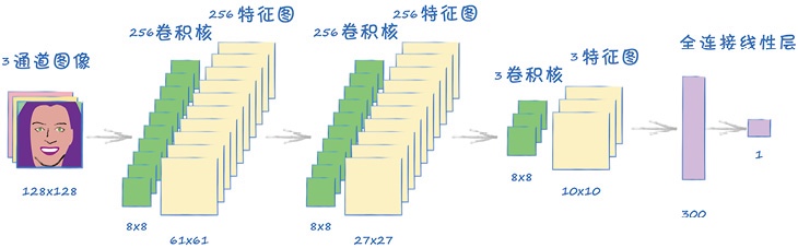
class Discriminator(nn.Module):
  def __init__(self):
    # 初始化pytorch父类
    super().__init__()
    # 定义神经网络层
    self.model = nn.Sequential(
        # 与其输入形状为 (1, 3, 128, 128)
        nn.Conv2d(3, 256, kernel_size=8, stride=2), # 输入3通道彩色图像，应用256个卷积核，输出256个特征图，卷积核大小8*8，步长2，因此输出特征图大小为61*61
        nn.BatchNorm2d(256),              # 对图层中的每个通道进行标准化
        nn.LeakyReLU(0.2),
        nn.Conv2d(256, 256, kernel_size=8, stride=2), # 输入256通道（256个特征图），应用256个卷积核，输出256个特征图，卷积核大小8*8，步长2，因此输出特征图大小为27*27
        nn.BatchNorm2d(256),               # 对图层中的每个通道进行标准化
        nn.LeakyReLU(0.2),
        nn.Conv2d(256, 3, kernel_size=8, stride=2),   # 输入256通道（256个特征图），应用3个卷积核，输出3个特征图，卷积核大小8*8，步长2，因此输出特征图大小为10*10
        nn.LeakyReLU(0.2),
        View(3*10*10),        # 输入（1，3，10，10）的三维特征图，转换为含100个值的一维张量
        nn.Linear(3*10*10, 1),    # 全连接层，将300个值所见到一个鉴别器的输出值
        nn.Sigmoid()
    )
    # 创建损失函数
    self.loss_function = nn.BCELoss()   # 二元交叉熵BCELoss()
    # 创建优化器，使用随机梯度下降
    self.optimiser = torch.optim.Adam(self.parameters(), lr=0.0001)   # 使用Adam优化器
    # 计数器和进程记录
    self.counter = 0
    self.progress = []
    pass
  def forward(self, inputs):
    # 直接运行模型
    return self.model(inputs)
  def train(self, inputs, targets):
    # 计算网络的输出
    outputs = self.forward(inputs)
    # 计算损失值
    loss = self.loss_function(outputs, targets)
    # 每训练10次增加计数器
    self.counter += 1
    if(self.counter % 10 == 0):
      self.progress.append(loss.item())
      pass
    if(self.counter % 10000 == 0):
      print("counter = ", self.counter)
      pass
    # 归零梯度，反向传播，并更新权重
    self.optimiser.zero_grad()
    loss.backward()
    self.optimiser.step()
    pass
  def plot_progress(self):  # 打印训练过程
    df = pandas.DataFrame(self.progress, columns=['loss'])
    df.plot(ylim=(0), figsize=(16, 8), alpha=0.1, marker='.', grid=True, yticks=(0, 0.25, 0.5, 1.0, 5.0))
    pass
  pass

测试鉴别器

%%time
# 测试鉴别器能否鉴别真实数据和随机噪声
# 训练鉴别器
D = Discriminator()
D.to(device)  # 将模型移到cuda设备
for image_data_tensor in celeba_dataset:
  # 真实数据
  D.train(image_data_tensor, torch.cuda.FloatTensor([1.0]))
  # 生成数据
  D.train(generate_random_image((1, 3, 128, 128)), torch.cuda.FloatTensor([0.0]))
  pass

# 绘制鉴别器的损失图
D.plot_progress()

# 运行鉴别器，检查其能否区分真实图像和随机图像
for i in range(4):
  image_data_tensor = celeba_dataset[random.randint(0, 20000)]
  print(D.forward(image_data_tensor).item())
  pass
for i in range(4):
  print(D.forward(generate_random_image((1, 3, 128, 128))).item())
  pass

生成器网络

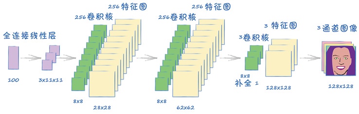
class Generator(nn.Module):
  def __init__(self):
    # 初始化pytorch父类
    super().__init__()
    # 定义神经网络层
    self.model = nn.Sequential(
        # 输入是一个一维数组（100个种子）
        nn.Linear(100, 3*11*11),  
        nn.LeakyReLU(0.2),   
        # 转换成四维
        View((1, 3, 11, 11)),
        nn.ConvTranspose2d(3, 256, kernel_size=8, stride=2),  # 转置卷积，256个卷积核
        nn.BatchNorm2d(256),
        nn.LeakyReLU(0.2),
        nn.ConvTranspose2d(256, 256, kernel_size=8, stride=2),
        nn.BatchNorm2d(256),
        nn.LeakyReLU(0.2),
        nn.ConvTranspose2d(256, 3, kernel_size=8, stride=2, padding=1),  # 因为输出要红绿蓝三通道，因此使用三个转置卷积核；padding用于从中间网格中去掉外围的方格
        nn.BatchNorm2d(3),
        nn.Sigmoid()  
        # 输出为 (1, 3, 128, 128)
    )
    # 不需要损失函数！！！
    # 创建优化器，使用随机梯度下降
    self.optimiser = torch.optim.Adam(self.parameters(), lr=0.0001)   # 使用Adam优化器
    # 计数器和进程记录
    self.counter = 0
    self.progress = []
    pass
  def forward(self, inputs):
    # 直接运行模型
    return self.model(inputs)
  def train(self, D, inputs, targets):
    # 计算网络的输出
    g_outputs = self.forward(inputs)
    # 训练生成器需要鉴别器的损失值
    # 将生成器网络的输出输入到鉴别器
    d_outputs = D.forward(g_outputs)
    # 计算鉴别器的损失值
    loss = D.loss_function(d_outputs, targets)
    # 每训练10次增加计数器
    self.counter += 1
    if(self.counter % 10 == 0):
      self.progress.append(loss.item())
      pass
    # 鉴别器训练中不打印，这样可以通过真实的训练数据更准确地反应训练进度
    # 归零梯度，反向传播，并更新权重
    self.optimiser.zero_grad()
    loss.backward()
    self.optimiser.step()
    pass
  def plot_progress(self):  # 打印训练过程
    df = pandas.DataFrame(self.progress, columns=['loss'])
    df.plot(ylim=(0), figsize=(16, 8), alpha=0.1, marker='.', grid=True, yticks=(0, 0.25, 0.5, 1.0, 5.0))
    pass
  pass

检查生成器输出

# 检查生成器的输出大小，并确保运行没有错误
G = Generator()
# 将模型转存到CUDA设备
G.to(device)
output = G.forward(generate_random_seed(100))
img = output.detach().permute(0, 2, 3, 1).view(128, 128, 3).cpu().numpy() # 用detach将输出图像与pytorch的计算图分离，存回CPU并转换成numpy数组
# 上面permute(0,2,3,1)将numpy数组（批量大小，通道数3，高，宽）重新排序为（批量大小，高，宽，通道数3）；view(128, 128, 3)则去掉了批量大小这一维度，将numpy转为三维张量（高，宽，通道数）
plt.imshow(img, interpolation='none', cmap='Blues')

训练GAN

%%time
# 创建鉴别器和生成器
D = Discriminator()
D.to(device)
G= Generator()
G.to(device)
epochs = 1
for epoch in range(epochs):
  print("epoch = ", epoch + 1)
  # 训练鉴别器和生成器
  for image_data_tensor in celeba_dataset:
    # 第一步：用真实样本训练鉴别器
    D.train(image_data_tensor, torch.cuda.FloatTensor([1.0]))
    # 第二步：用生成样本训练鉴别器
    # 使用detach()以避免计算生成器G中的梯度，节省计算成本
    D.train(G.forward(generate_random_seed(100)).detach(), torch.cuda.FloatTensor([0.0]))
    # 第三步：训练生成器
    G.train(D, generate_random_seed(100), torch.cuda.FloatTensor([1.0]))
    pass
  pass

# 绘制鉴别器的损失图
D.plot_progress()

# 绘制生成器的损失图
G.plot_progress()
# 实际上，鉴别器和生成器的二元交叉熵损失值最理想的情况是ln2=0.693

运行生成器

# 从训练好的生成器绘制一些输出
# 在3行2列的网格中绘制生成图像（检查生成图像的多样性）
f, axarr = plt.subplots(2, 3, figsize=(16, 8))
for i in range(2):
  for j in range(3):
    output = G.forward(generate_random_seed(100))
    img = output.detach().permute(0, 2, 3, 1).view(128, 128, 3).cpu().numpy()
    axarr[i, j].imshow(img, interpolation='none', cmap='Blues')
    pass
  pass

条件式 GAN - MNIST 生成指定数字图像

16_cgan_mnist.ipynb

• 挂载驱动器以访问 google drive 中的文件 ```python

  mount Drive to access data files

from google.colab import drive drive.mount(‘./mount’)

- 导入包
```python
import torch
import torch.nn as nn
from torch.utils.data import Dataset
import pandas, numpy, random
import matplotlib.pyplot as plt

数据类

class MnistDataset(Dataset):  # 对于继承自Dataset的数据集，需要提供__len__()函数和__getitem__()函数
  def __init__(self, csv_file):
    self.data_df = pandas.read_csv(csv_file, header=None)
    pass
  def __len__(self):  # 获取数据集大小（返回数据集中的项目总数）
    return len(self.data_df)
  def __getitem__(self, index):   # 通过索引获取数据集中的项目
    # 目标图像（标签）
    label = self.data_df.iloc[index, 0]
    target = torch.zeros((10))
    target[label] = 1.0 # 转换为one-hot形式的标签向量
    # 图像数据，取值范围是0-255，标准化为0-1
    image_values = torch.FloatTensor(self.data_df.iloc[index, 1:].values) / 255.0
    # 返回标签、图像数据张量以及目标张量
    return label, image_values, target
  def plot_image(self, index):  # 通过索引号，绘制对应编号的图
    img = self.data_df.iloc[index, 1:].values.reshape(28, 28)
    plt.title("label = " + str(self.data_df.iloc[index, 0]))
    plt.imshow(img, interpolation='none', cmap='Blues')
    pass
  pass

# 测试Dataset类是否可以正常工作
# 加载数据
mnist_dataset = MnistDataset('mount/My Drive/Colab Notebooks/pytorch_gan/mnist_data/mnist_train.csv')

# 检查数据包含图像
mnist_dataset.plot_image(17)

生成随机数据的辅助函数

# 生成随机数据的函数
def generate_random_image(size):
    random_data = torch.rand(size)
    return random_data
def generate_random_seed(size):
    random_data = torch.randn(size)
    return random_data
# size here must only be an integer
def generate_random_one_hot(size):
    label_tensor = torch.zeros((size))
    random_idx = random.randint(0,size-1)
    label_tensor[random_idx] = 1.0
    return label_tensor

鉴别器类

class Discriminator(nn.Module):
  def __init__(self):
    # 初始化pytorch父类
    super().__init__()
    # 定义神经网络层
    self.model = nn.Sequential(
        nn.Linear(784+10, 200), # 输入：图像张量28*28=784 + 标签张量长度10
        nn.LeakyReLU(0.02),
        nn.LayerNorm(200),
        nn.Linear(200, 1),
        nn.Sigmoid()
    )
    # 创建损失函数
    self.loss_function = nn.BCELoss() 
    # 创建优化器，使用随机梯度下降
    self.optimiser = torch.optim.Adam(self.parameters(), lr=0.0001)   # 改良4：使用Adam优化器
    # 计数器和进程记录
    self.counter = 0
    self.progress = []
    pass
  def forward(self, image_tensor, label_tensor):  # 扩展forward()函数，使其同时接收图像张量和标签张量，并将它们拼接起来
    # 拼接种子和标签
    inputs = torch.cat((image_tensor, label_tensor))
    return self.model(inputs)
  def train(self, inputs, label_tensor, targets): # 扩展：接收标签张量
    # 计算网络的输出
    outputs = self.forward(inputs, label_tensor)  # 同时接收图像张量和标签张量
    # 计算损失值
    loss = self.loss_function(outputs, targets)
    # 每训练10次增加计数器
    self.counter += 1
    if(self.counter % 10 == 0):
      self.progress.append(loss.item())
      pass
    if(self.counter % 10000 == 0):
      print("counter = ", self.counter)
      pass
    # 归零梯度，反向传播，并更新权重
    self.optimiser.zero_grad()
    loss.backward()
    self.optimiser.step()
    pass
  def plot_progress(self):  # 打印训练过程
    df = pandas.DataFrame(self.progress, columns=['loss'])
    df.plot(ylim=(0), figsize=(16, 8), alpha=0.1, marker='.', grid=True, yticks=(0, 0.25, 0.5, 1.0, 5.0))
    pass
  pass

测试鉴别器

%%time
# 测试鉴别器，确保其至少能将真实图像与随机噪声区分开
# 训练鉴别器，奖励鉴别器将真实的训练数据判别为真，也就是输出1.0；将伪造的生成数据判别为假，也就是输出0.0
D = Discriminator()
for label, image_data_tensor, label_tensor in mnist_dataset:
  # 真实数据
  D.train(image_data_tensor, label_tensor, torch.FloatTensor([1.0]))
  # 生成数据
  D.train(generate_random_image(784), generate_random_one_hot(10), torch.FloatTensor([0.0]))
  pass

# 绘制训练过程中的损失值变化
D.plot_progress()
# 损失之下降并一直保持接近0的值，这正是我们希望达到的效果

# 随机选取一些训练集中的图像和随机噪声图像，分别作为输入来测试训练后的鉴别器
for i in range(4):
  label, image_data_tensor, label_tensor = mnist_dataset[random.randint(0, 6000)]
  print(D.forward(image_data_tensor, label_tensor).item())
  pass
for i in range(4):
  print(D.forward(generate_random_image(784), generate_random_one_hot(10)).item())
  pass

生成器类

条件式GAN架构：要让训练后的GAN生成器生成一个指定数字的图像，因此生成器和鉴别器的输入都在图像数据的基础上加入了类型标签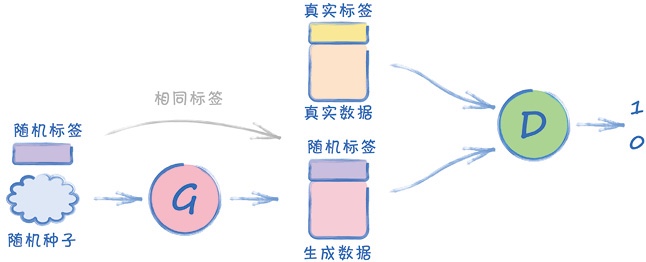

class Generator(nn.Module):
  def __init__(self):
    # 初始化pytorch父类
    super().__init__()
    # 定义神经网络层
    self.model = nn.Sequential(
        nn.Linear(100+10, 200),
        nn.LeakyReLU(0.02),
        nn.LayerNorm(200),
        nn.Linear(200, 784),
        nn.Sigmoid()
    )
    # 不需要损失函数！！！
    # 创建优化器，使用随机梯度下降
    self.optimiser = torch.optim.Adam(self.parameters(), lr=0.0001)
    # 计数器和进程记录
    self.counter = 0
    self.progress = []
    pass
  def forward(self, seed_tensor, label_tensor):
    # 拼接种子和标签
    inputs = torch.cat((seed_tensor, label_tensor))
    return self.model(inputs)
  def train(self, D, inputs, label_tensor, targets):
    # 计算网络的输出
    g_outputs = self.forward(inputs, label_tensor)
    # 训练生成器需要鉴别器的损失值
    # 将生成器网络的输出输入到鉴别器
    d_outputs = D.forward(g_outputs, label_tensor)
    # 计算鉴别器的损失值
    loss = D.loss_function(d_outputs, targets)
    # 每训练10次增加计数器
    self.counter += 1
    if(self.counter % 10 == 0):
      self.progress.append(loss.item())
      pass
    # 鉴别器训练中不打印，这样可以通过真实的训练数据更准确地反应训练进度
    # 归零梯度，反向传播，并更新权重
    self.optimiser.zero_grad()
    loss.backward()
    self.optimiser.step()
    pass
  # 这个函数不应该放在类里把，应该单独拎出来，下面imshow那个G.forward，G是哪来的？
  def plot_images(self, label):
    label_tensor = torch.zeros((10))
    label_tensor[label] = 1.0
    # 在3行2列的网格中生成图像
    f, axarr = plt.subplots(2, 3, figsize=(16, 8))
    for i in range(2):
      for j in range(3):
        axarr[i, j].imshow(G.forward(generate_random_seed(100), label_tensor).detach().cpu().numpy().reshape(28, 28), interpolation='none', cmap='Blues')
        pass
      pass
    pass
  def plot_progress(self):  # 打印训练过程
    df = pandas.DataFrame(self.progress, columns=['loss'])
    df.plot(ylim=(0), figsize=(16, 8), alpha=0.1, marker='.', grid=True, yticks=(0, 0.25, 0.5, 1.0, 5.0))
    pass
  pass

检查生成器输出

# 训练生成器前，先检查生成器输出格式是否正确
G = Generator()
output = G.forward(generate_random_seed(100), generate_random_one_hot(10))
img = output.detach().numpy().reshape(28, 28)
plt.imshow(img, interpolation='none', cmap='Blues')

训练GAN

%%time
# 训练GAN
# 创建鉴别器和生成器
D = Discriminator()
G = Generator()
epochs = 4
# 训练鉴别器和生成器
for epoch in range(epochs):
  print("epoch = ", epoch + 1)
  for label, image_data_tensor, label_tensor in mnist_dataset:
    # 第一步：用真实样本训练鉴别器
    D.train(image_data_tensor, label_tensor, torch.FloatTensor([1.0]))
    # 为鉴别器生成一个随机独热标签（用生成图像训练鉴别器时，对生成器和鉴别器输入同一标签张量）
    random_label = generate_random_one_hot(10)
    # 第二步：用生成样本训练鉴别器
    # 使用detach()以避免计算生成器G中的梯度，节省计算成本
    D.train(G.forward(generate_random_seed(100), random_label).detach(), random_label, torch.FloatTensor([0.0]))
    # 为生成器另外生成一个随机独热标签
    random_label = generate_random_one_hot(10)
    # 第三步：训练生成器（输入鉴别器对象和随机单值输入来训练生成器）
    G.train(D, generate_random_seed(100), random_label, torch.FloatTensor([1.0]))
    pass
  pass

# 绘制鉴别器在训练中的损失值变化图
D.plot_progress()
# 损失值迅速下降到接近于0，并一直保持在很低的位置。训练期间，损失值偶尔发生跳跃。这说明生成器和鉴别器之间仍然没有取得平衡

# 绘制生成器训练过程中的损失值变化图
G.plot_progress()
# 损失值先是上升，表示在训练早期生成器落后于鉴别器。之后，损失值下降并保持在3左右。记住，与MSELoss不同，BCELoss没有1.0的上限

运行生成器

# 试验训练后的生成器会生成什么样的图像
# 由于不同的随机种子应当生成不同的图像，所以绘制多幅输出图像并查看
label = 9
label_tensor = torch.zeros((10))
label_tensor[label] = 1.0
# 在3行2列的网格中生成图像
f, axarr = plt.subplots(2, 3, figsize=(16, 8))
for i in range(2):
  for j in range(3):
    output = G.forward(generate_random_seed(100), label_tensor)
    img = output.detach().cpu().numpy().reshape(28, 28)
    axarr[i, j].imshow(img, interpolation='none', cmap='Blues')
    pass
  pass
# 由图可知，生成的图像不是随机噪声，而是有某种形状
# 但这些图像看起来都相同，这种现象称为“模式崩溃”

总结

• 训练 GAN 时的理想状态：生成器与鉴别器达到平衡，生成器已经学会了生成看起来足以以假乱真的数据，使得鉴别器无法区分真实数据与生成器生成的数据

• 训练 GAN 时的理想损失值：（即生成器和鉴别器达到平衡时的损失值）

  • 均方误差 MSE Loss：0.25
    • 即鉴别器无法从伪造数据中识别真实数据，就无法确定输出0.0还是1.0，索性就输出0.5，因此均方误差为
  • 二元交叉熵 BCE Loss：ln2 ≈ 0.693

• GAN 不会学习记忆训练数据中的实例，GAN 学习的是训练数据中每个元素出现的可能性（即概率分布）

• 模式崩溃：

  • eg. 使用 MNIST 数据集训练 GAN，希望生成所有 10 个数字，也就是说希望能学习到所有 10 个数字图像的概率分布
  • 但，有可能训练出的GAN只会生成其中一种数字，也就是模式崩溃，即生成器只学会了一类图像的概率分布

• 梯度下降并不适合对抗博弈