有了前面的基础,我们就可以利用PySpark进行数据的分析与挖掘,而通常我们需要花费80%——90%的时间用于数据的预处理,这是我们后续建模开发的基础,本文将基于PySpark对大规模数据预处理从实际业务场景出发进行分析,从而更接地气!!!
1 重复数据
spark 2.0+
df = spark.createDataFrame([(1, 144.5, 5.9, 33, 'M'),(2, 167.2, 5.4, 45, 'M'),(3, 124.1, 5.2, 23, 'F'),(4, 144.5, 5.9, 33, 'M'),(5, 133.2, 5.7, 54, 'F'),(3, 124.1, 5.2, 23, 'F'),(5, 129.2, 5.3, 42, 'M')],['id','weight','height','age','gender'])
spark 1.6.2
df = sqlContext.createDataFrame([(1, 144.5, 5.9, 33, 'M'),(2, 167.2, 5.4, 45, 'M'),(3, 124.1, 5.2, 23, 'F'),(4, 144.5, 5.9, 33, 'M'),(5, 133.2, 5.7, 54, 'F'),(3, 124.1, 5.2, 23, 'F'),(5, 129.2, 5.3, 42, 'M')],['id','weight','height','age','gender'])
1.1 检查重复数据
用 .distinct() 完全相同的两行或多行去重
print('Count of rows: {0}'.format(df.count()))print('Count of distinct rows: {0}'.format(df.distinct().count()))Count of rows: 7Count of distinct rows: 6
用 .dropDuplicates(…) 方法去除重复行,具体用法可以参考本文集 Pyspark.SQL模块介绍
df = df.dropDuplicates()df.show()+---+------+------+---+------+| id|weight|height|age|gender|+---+------+------+---+------+| 5| 129.2| 5.3| 42| M|| 4| 144.5| 5.9| 33| M|| 3| 124.1| 5.2| 23| F|| 2| 167.2| 5.4| 45| M|| 1| 144.5| 5.9| 33| M|| 5| 133.2| 5.7| 54| F|+---+------+------+---+------+
除了ID字段外的消除重复行
print('Count of ids: {0}'.format(df.count()))#print('Count of distinct ids: {0}'.format(df.select([c for c in df.columns if c != 'id']).distinct().count()))print('Count of distinct ids:{0}'.format(df.select(["weight","height","age","gender"]).distinct().count()))Count of ids: 6Count of distinct ids:5
使用 .dropDuplicates(…) 处理重复行,但是添加 subset 参数
# df = df.dropDuplicates(subset=[c for c in df.columns if c != 'id'])df =df.dropDuplicates(["weight","height","age","gender"])df.show()+---+------+------+---+------+| id|weight|height|age|gender|+---+------+------+---+------+| 5| 133.2| 5.7| 54| F|| 4| 144.5| 5.9| 33| M|| 2| 167.2| 5.4| 45| M|| 5| 129.2| 5.3| 42| M|| 3| 124.1| 5.2| 23| F|+---+------+------+---+------+
利用.agg(…)函数计算ID的总数和ID唯一个数
import pyspark.sql.functions as fndf.agg(fn.count('id').alias('id_count'),fn.countDistinct('id').alias('id_distinct')).show()+--------+-----------+|id_count|id_distinct|+--------+-----------+| 5| 4|+--------+-----------+
给每一行一个唯一的ID号,相当于新增一列数字
df.withColumn('new_id', fn.monotonically_increasing_id()).show()+---+------+------+---+------+------------+| id|weight|height|age|gender| new_id|+---+------+------+---+------+------------+| 5| 133.2| 5.7| 54| F|283467841536|| 4| 144.5| 5.9| 33| M|352187318272|| 2| 167.2| 5.4| 45| M|386547056640|| 5| 129.2| 5.3| 42| M|438086664192|| 3| 124.1| 5.2| 23| F|463856467968|+---+------+------+---+------+------------+
1.2 缺失值观察
df_miss = sqlContext.createDataFrame([(1, 143.5, 5.6, 28, 'M', 100000),(2, 167.2, 5.4, 45, 'M', None),(3, None , 5.2, None, None, None),(4, 144.5, 5.9, 33, 'M', None),(5, 133.2, 5.7, 54, 'F', None),(6, 124.1, 5.2, None, 'F', None),(7, 129.2, 5.3, 42, 'M', 76000),], ['id', 'weight', 'height', 'age', 'gender', 'income'])df_miss.show()+---+------+------+----+------+------+| id|weight|height| age|gender|income|+---+------+------+----+------+------+| 1| 143.5| 5.6| 28| M|100000|| 2| 167.2| 5.4| 45| M| null|| 3| null| 5.2|null| null| null|| 4| 144.5| 5.9| 33| M| null|| 5| 133.2| 5.7| 54| F| null|| 6| 124.1| 5.2|null| F| null|| 7| 129.2| 5.3| 42| M| 76000|+---+------+------+----+------+------+
统计每行缺失值的个数
df_miss.rdd.\map(lambda row:(sum([c == None for c in row]),row['id'])).\sortByKey(ascending=False).collect() #(缺失值个数,行号)[(4, 3), (2, 6), (1, 2), (1, 4), (1, 5), (0, 1), (0, 7)]df_miss.where('id = 3').show()+---+------+------+----+------+------+| id|weight|height| age|gender|income|+---+------+------+----+------+------+| 3| null| 5.2|null| null| null|+---+------+------+----+------+------+
每一列缺失的观测数据的百分比
# fn.count(c) / fn.count('*') 为每列字段非缺失的记录数占比# fn.count('*') *表示列名的位置,指示该列方法计算所有的列# .agg(* *之前的列指示,.agg(...)方法将该列表处理为一组独立的参数传递给函数df_miss.agg(*[(1.00 - (fn.count(c) / fn.count('*'))).alias(c + '_missing') for c in df_miss.columns]).show()+----------+------------------+--------------+------------------+------------------+------------------+|id_missing| weight_missing|height_missing| age_missing| gender_missing| income_missing|+----------+------------------+--------------+------------------+------------------+------------------+| 0.0|0.1428571428571429| 0.0|0.2857142857142857|0.1428571428571429|0.7142857142857143|+----------+------------------+--------------+------------------+------------------+------------------+
移除income列,因为income列大部分是缺失值,缺失值占比达到71%
df_miss_no_income = df_miss.select([c for c in df_miss.columns if c != 'income'])df_miss_no_income.show()+---+------+------+----+------+| id|weight|height| age|gender|+---+------+------+----+------+| 1| 143.5| 5.6| 28| M|| 2| 167.2| 5.4| 45| M|| 3| null| 5.2|null| null|| 4| 144.5| 5.9| 33| M|| 5| 133.2| 5.7| 54| F|| 6| 124.1| 5.2|null| F|| 7| 129.2| 5.3| 42| M|+---+------+------+----+------+
使用.dropna(…) 移除方法,thresh(设定移除数的阈值)
df_miss_no_income.dropna(thresh=3).show()+---+------+------+----+------+| id|weight|height| age|gender|+---+------+------+----+------+| 1| 143.5| 5.6| 28| M|| 2| 167.2| 5.4| 45| M|| 4| 144.5| 5.9| 33| M|| 5| 133.2| 5.7| 54| F|| 6| 124.1| 5.2|null| F|| 7| 129.2| 5.3| 42| M|+---+------+------+----+------+
使用.fillna(…) 方法,填充观测数据.
means = df_miss_no_income.agg(*[fn.mean(c).alias(c) for c in df_miss_no_income.columns if c != 'gender']).toPandas().to_dict('records')[0]# gender单独处理means['gender'] = 'missing'df_miss_no_income.fillna(means).show()+---+-------------+------+---+-------+| id| weight|height|age| gender|+---+-------------+------+---+-------+| 1| 143.5| 5.6| 28| M|| 2| 167.2| 5.4| 45| M|| 3|140.283333333| 5.2| 40|missing|| 4| 144.5| 5.9| 33| M|| 5| 133.2| 5.7| 54| F|| 6| 124.1| 5.2| 40| F|| 7| 129.2| 5.3| 42| M|+---+-------------+------+---+-------+
1.3 离群值Outliers(异常数据)
df_outliers = sqlContext.createDataFrame([(1, 143.5, 5.3, 28),(2, 154.2, 5.5, 45),(3, 342.3, 5.1, 99),(4, 144.5, 5.5, 33),(5, 133.2, 5.4, 54),(6, 124.1, 5.1, 21),(7, 129.2, 5.3, 42),], ['id', 'weight', 'height', 'age'])df_outliers.show()+---+------+------+---+| id|weight|height|age|+---+------+------+---+| 1| 143.5| 5.3| 28|| 2| 154.2| 5.5| 45|| 3| 342.3| 5.1| 99|| 4| 144.5| 5.5| 33|| 5| 133.2| 5.4| 54|| 6| 124.1| 5.1| 21|| 7| 129.2| 5.3| 42|+---+------+------+---+
使用之前列出的定义来标记离群值
# approxQuantile(col, probabilities, relativeError) New in version 2.0.cols = ['weight', 'height', 'age']bounds = {}for col in cols:quantiles = df_outliers.approxQuantile(col, [0.25, 0.75], 0.05)IQR = quantiles[1] - quantiles[0]bounds[col] = [quantiles[0] - 1.5 * IQR,quantiles[1] + 1.5 * IQR]
bounds字典保存了每个特征的上下界限
bounds{'age': [9.0, 51.0],'height': [4.8999999995, 5.6],'weight': [115.0, 146.8499999997]}
标记样本数据的离群值
# 按位或运算符:只要对应的两个二进位有一个为1时,结果位就为1。outliers = df_outliers.select(*['id'] + [((df_outliers[c] < bounds[c][0]) | (df_outliers[c] > bounds[c][1])).alias(c + '_o') \for c in cols \]\)outliers.show()+---+--------+--------+-----+| id|weight_o|height_o|age_o|+---+--------+--------+-----+| 1| false| false|false|| 2| true| false|false|| 3| true| false| true|| 4| false| false|false|| 5| false| false| true|| 6| false| false|false|| 7| false| false|false|+---+--------+--------+-----+
列出weight和age与其他分部明显不同的部分(离群值)
df_outliers = df_outliers.join(outliers, on='id')df_outliers.filter('weight_o').select('id', 'weight').show()df_outliers.filter('age_o').select('id', 'age').show()+---+------+| id|weight|+---+------+| 3| 342.3|| 2| 154.2|+---+------++---+---+| id|age|+---+---+| 5| 54|| 3| 99|+---+---+
通过上述方法即可获得快速清洗数据(重复值、缺失值和离群值)
2 熟悉理解你的数据
2.1描述性统计——EDA
加载数据并且转换为Spark DatFrame
# pyspark.sql.types显示了所有的我们可以使用的数据类型,IntegerType()和FloatType()from pyspark.sql import typesfraud = sc.textFile('file:///root/ydzhao/PySpark/Chapter04/ccFraud.csv.gz') # 信用卡欺诈数据集header = fraud.first()header'"custID","gender","state","cardholder","balance","numTrans","numIntlTrans","creditLine","fraudRisk"'fraud.take(3)['"custID","gender","state","cardholder","balance","numTrans","numIntlTrans","creditLine","fraudRisk"','1,1,35,1,3000,4,14,2,0','2,2,2,1,0,9,0,18,0']fraud.count()10000001# (1) 去除标题行数据,每个元素转换成整型Integer,还是RDDfraud = fraud.filter(lambda row: row != header).map(lambda row: [int(x) for x in row.split(',')])fraud.take(3)[[1, 1, 35, 1, 3000, 4, 14, 2, 0],[2, 2, 2, 1, 0, 9, 0, 18, 0],[3, 2, 2, 1, 0, 27, 9, 16, 0]]# (2) 创建DataFrame模式# h[1:-1]代表第一行到最后一行schema = [*[types.StructField(h[1:-1], types.IntegerType(), True) for h in header.split(',')]]schema = types.StructType(schema)# (3) 创建DataFrame# spark2.0+# fraud_df = spark.createDataFrame(fraud, schema)# spark1.6.2fraud_df = sqlContext.createDataFrame(fraud, schema)fraud_df.printSchema()root|-- custID: integer (nullable = true)|-- gender: integer (nullable = true)|-- state: integer (nullable = true)|-- cardholder: integer (nullable = true)|-- balance: integer (nullable = true)|-- numTrans: integer (nullable = true)|-- numIntlTrans: integer (nullable = true)|-- creditLine: integer (nullable = true)|-- fraudRisk: integer (nullable = true)fraud_df.show()+------+------+-----+----------+-------+--------+------------+----------+---------+|custID|gender|state|cardholder|balance|numTrans|numIntlTrans|creditLine|fraudRisk|+------+------+-----+----------+-------+--------+------------+----------+---------+| 1| 1| 35| 1| 3000| 4| 14| 2| 0|| 2| 2| 2| 1| 0| 9| 0| 18| 0|| 3| 2| 2| 1| 0| 27| 9| 16| 0|| 4| 1| 15| 1| 0| 12| 0| 5| 0|| 5| 1| 46| 1| 0| 11| 16| 7| 0|| 6| 2| 44| 2| 5546| 21| 0| 13| 0|| 7| 1| 3| 1| 2000| 41| 0| 1| 0|| 8| 1| 10| 1| 6016| 20| 3| 6| 0|| 9| 2| 32| 1| 2428| 4| 10| 22| 0|| 10| 1| 23| 1| 0| 18| 56| 5| 0|| 11| 1| 46| 1| 4601| 54| 0| 4| 0|| 12| 1| 10| 1| 3000| 20| 0| 2| 0|| 13| 1| 6| 1| 0| 45| 2| 4| 0|| 14| 2| 38| 1| 9000| 41| 3| 8| 0|| 15| 1| 27| 1| 5227| 60| 0| 17| 0|| 16| 1| 44| 1| 0| 22| 0| 5| 0|| 17| 2| 18| 1| 13970| 20| 0| 13| 0|| 18| 1| 35| 1| 3113| 13| 6| 8| 0|| 19| 1| 5| 1| 9000| 20| 2| 8| 0|| 20| 2| 31| 1| 1860| 21| 10| 8| 0|+------+------+-----+----------+-------+--------+------------+----------+---------+only showing top 20 rows
使用.groupby(…) 方法计算性别列的使用频率 我们所面对的样本一个性别比例失衡的样本.
fraud_df.groupby('gender').count().show()+------+-------+|gender| count|+------+-------+| 1|6178231|| 2|3821769|+------+-------+
使用describe()方法进行数值统计
desc = fraud_df.describe(['balance', 'numTrans', 'numIntlTrans'])desc.show()+-------+-----------------+------------------+-----------------+|summary| balance| numTrans| numIntlTrans|+-------+-----------------+------------------+-----------------+| count| 10000000| 10000000| 10000000|| mean| 4109.9199193| 28.9351871| 4.0471899|| stddev|3996.847309737077|26.553781024522852|8.602970115863767|| min| 0| 0| 0|| max| 41485| 100| 60|+-------+-----------------+------------------+-----------------+
检查balance偏度(skewness)
fraud_df.agg({'balance': 'skewness'}).show()+------------------+| skewness(balance)|+------------------+|1.1818315552996432|+------------------+
2.2 相关性
目前 .corr()方法仅仅支持Pearson相关性系数,且两两相关性。
当然你可以把Spark DataFrame 转换为Python的DataFrame之后,你就可以随便怎么弄了,但是开销可能会很大,由数据量决定。期待后续版本的更新。
fraud_df.corr('balance', 'numTrans')
创建相关系数矩阵
numerical = ['balance', 'numTrans', 'numIntlTrans']n_numerical = len(numerical)corr = []for i in range(0, n_numerical):temp = [None] * ifor j in range(i, n_numerical):temp.append(fraud_df.corr(numerical[i], numerical[j]))corr.append(temp)corr[[1.0, 0.00044523140172659576, 0.00027139913398184604],[None, 1.0, -0.0002805712819816179],[None, None, 1.0]]
2.3 数据可视化
加载matplotlib 和 bokeh包,只会调用python的解释器
%matplotlib inlineimport matplotlib.pyplot as pltplt.style.use('ggplot')import bokeh.charts as chrtfrom bokeh.io import output_notebookoutput_notebook()Loading BokehJS ...
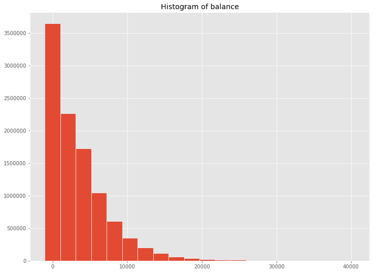
2.3.1 直方图Histograms
方法一 聚集工作节点中的数据并返回一个汇总bins列表和直方图每个bin中的计数给驱动(适用大数据集)
(1) 先对数据进行聚合
hists = fraud_df.select('balance').rdd.flatMap(lambda row: row).histogram(20)type(hists)tuple
(2)
使用matplotlib绘制直方图
data = {'bins': hists[0][:-1],'freq': hists[1]}fig = plt.figure(figsize=(12,9))ax = fig.add_subplot(1, 1, 1)ax.bar(data['bins'], data['freq'], width=2000)ax.set_title('Histogram of balance')plt.savefig('balance.png', dpi=300)
使用Bokeh绘制直方图
b_hist = chrt.Bar(data, values='freq', label='bins', title='Histogram of balance')chrt.show(b_hist)
方法二 所有数据给驱动程序(适用于小数据集) 当然方法一是性能更好的
data_driver = {'obs': fraud_df.select('balance').rdd.flatMap(lambda row: row).collect()}fig = plt.figure(figsize=(12,9))ax = fig.add_subplot(1, 1, 1)ax.hist(data_driver['obs'], bins=20)ax.set_title('Histogram of balance using .hist()')plt.savefig('balance_hist.png', dpi=300)

使用Bokeh绘制直方图
b_hist_driver = chrt.Histogram(data_driver, values='obs', title='Histogram of balance using .Histogram()', bins=20)chrt.show(b_hist_driver)
2.3.2 特征值之间的交互
10000000条数据先抽样0.02%
data_sample = fraud_df.sampleBy('gender', {1: 0.0002, 2: 0.0002}).select(numerical)data_sample.show()+-------+--------+------------+|balance|numTrans|numIntlTrans|+-------+--------+------------+| 0| 15| 0|| 4000| 3| 0|| 6000| 21| 50|| 0| 28| 10|| 8630| 100| 0|| 4000| 17| 0|| 5948| 76| 0|| 3000| 9| 4|| 0| 5| 0|| 1588| 55| 0|| 3882| 87| 0|| 1756| 12| 0|| 4000| 4| 0|| 0| 10| 0|| 5000| 17| 0|| 4188| 50| 0|| 3141| 2| 1|| 8000| 52| 5|| 9000| 40| 0|| 2423| 11| 1|+-------+--------+------------+only showing top 20 rowsdata_multi = dict([(x, data_sample.select(x).rdd.flatMap(lambda row: row).collect())for x in numerical])sctr = chrt.Scatter(data_multi, x='balance', y='numTrans')chrt.show(sctr)

若有收获,就点个赞吧
0 人点赞
