由于MLlib现在已经处于维护状态（以后很可能被弃用），从Spark2.0开始，ML是主要的机器学习库，它对DataFrame进行操作，而不像MLlib那样对RDD进行操作。因此，本文将对最新版Spark2.2.0的机器学习包ML的各个功能模块进行详细分析，并以实际业务构建整个大规模数据的机器学习框架。

参考地址：spark.apache.org/docs/latest/api/python/pyspark.ml.html

pyspark.ml package

• ML Pipeline APIs
• pyspark.ml.param module
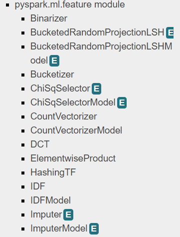
• pyspark.ml.feature module
• pyspark.ml.classification module
• pyspark.ml.clustering module
• pyspark.ml.linalg module
• pyspark.ml.recommendation module
• pyspark.ml.regression module
• pyspark.ml.stat module
• pyspark.ml.tuning module
• pyspark.ml.evaluation module
• pyspark.ml.fpm module
• pyspark.ml.util module

1.ML模块包括机器学习三个核心功能：

（1）数据准备：特征提取、变换、选择、分类特征的散列和自然语言处理等等；

（2）机器学习方法：实现了一些流行和高级的回归，分类和聚类算法；

（3）实用程序：统计方法，如描述性统计、卡方检验、线性代数（稀疏稠密矩阵和向量）和模型评估方法。

目前ML模块还处于不断发展中，但是已经可以满足我们的基础数据科学任务。
注意：官网上，标注“E”为测试阶段，不稳定，可能会产生错误失败。

2.ML模块三个抽象类

转换器（Transformer）、评估器（Estimator）和管道（Pipeline）

2.1 转换器

pyspark.ml.Transformer
通常通过将一个新列附加到DataFrame来转换数据。
当从转换器的抽象类派生时，每个新的转换器类需要实现.transform()方法,该方法要求传递一个要被转换的DataFrame，该参数通常是第一个也是唯一的一个强制性参数。

transform(dataset, params=None)
          Transforms the input dataset with optional parameters（使用可选参数转换输入数据集。）.      
Parameters:    
**dataset** – input dataset, which is an instance of pyspark.sql.DataFrame
**params** – an optional param map that overrides embedded params.
Returns:    transformed dataset

pyspark.ml.feature模块提供了许多的转换器：

pyspark.ml.feature.Binarizer(self, threshold=0.0, inputCol=None, outputCol=None)
根据指定的阈值将连续变量转换为对应的二进制

>>> df = spark.createDataFrame([(0.5,)], ["values"])
>>> binarizer = Binarizer(threshold=1.0, inputCol="values", outputCol="features")
>>> binarizer.transform(df).head().features
0.0
>>> binarizer.setParams(outputCol="freqs").transform(df).head().freqs
0.0
>>> params = {binarizer.threshold: -0.5, binarizer.outputCol: "vector"}
>>> binarizer.transform(df, params).head().vector
1.0
>>> binarizerPath = temp_path + "/binarizer"
>>> binarizer.save(binarizerPath)
>>> loadedBinarizer = Binarizer.load(binarizerPath)
>>> loadedBinarizer.getThreshold() == binarizer.getThreshold()
True

pyspark.ml.feature.Bucketizer(self, splits=None, inputCol=None, outputCol=None, handleInvalid=”error”)
与Binarizer类似，该方法根据阈值列表（分割的参数），将连续变量转换为多项值（连续变量离散化到指定的范围区间）

>>> values = [(0.1,), (0.4,), (1.2,), (1.5,), (float("nan"),), (float("nan"),)]
>>> df = spark.createDataFrame(values, ["values"])
>>> bucketizer = Bucketizer(splits=[-float("inf"), 0.5, 1.4, float("inf")],
...     inputCol="values", outputCol="buckets")
>>> bucketed = bucketizer.setHandleInvalid("keep").transform(df).collect()
>>> len(bucketed)
6
>>> bucketed[0].buckets
0.0
>>> bucketed[1].buckets
0.0
>>> bucketed[2].buckets
1.0
>>> bucketed[3].buckets
2.0
>>> bucketizer.setParams(outputCol="b").transform(df).head().b
0.0
>>> bucketizerPath = temp_path + "/bucketizer"
>>> bucketizer.save(bucketizerPath)
>>> loadedBucketizer = Bucketizer.load(bucketizerPath)
>>> loadedBucketizer.getSplits() == bucketizer.getSplits()
True
>>> bucketed = bucketizer.setHandleInvalid("skip").transform(df).collect()
>>> len(bucketed)
4

pyspark.ml.feature.ChiSqSelector(self, numTopFeatures=50, featuresCol=”features”, outputCol=None, labelCol=”label”, selectorType=”numTopFeatures”, percentile=0.1, fpr=0.05, fdr=0.05, fwe=0.05)
对于分类目标变量（思考分类模型），此功能允许你选择预定义数量的特征（由numTopFeatures参数进行参数化），以便最好地说明目标的变化。该方法需要两部：需要.fit()——可以计算卡方检验，调用.fit()方法，将DataFrame作为参数传入返回一个ChiSqSelectorModel对象，然后可以使用该对象的.transform()方法来转换DataFrame。默认情况下，选择方法是numTopFeatures，默认顶级要素数设置为50。

>>> from pyspark.ml.linalg import Vectors
>>> df = spark.createDataFrame(
...    [(Vectors.dense([0.0, 0.0, 18.0, 1.0]), 1.0),
...     (Vectors.dense([0.0, 1.0, 12.0, 0.0]), 0.0),
...     (Vectors.dense([1.0, 0.0, 15.0, 0.1]), 0.0)],
...    ["features", "label"])
>>> selector = ChiSqSelector(numTopFeatures=1, outputCol="selectedFeatures")
>>> model = selector.fit(df)
>>> model.transform(df).head().selectedFeatures
DenseVector([18.0])
>>> model.selectedFeatures
[2]
>>> chiSqSelectorPath = temp_path + "/chi-sq-selector"
>>> selector.save(chiSqSelectorPath)
>>> loadedSelector = ChiSqSelector.load(chiSqSelectorPath)
>>> loadedSelector.getNumTopFeatures() == selector.getNumTopFeatures()
True
>>> modelPath = temp_path + "/chi-sq-selector-model"
>>> model.save(modelPath)
>>> loadedModel = ChiSqSelectorModel.load(modelPath)
>>> loadedModel.selectedFeatures == model.selectedFeatures
True

pyspark.ml.feature.CountVectorizer(self, minTF=1.0, minDF=1.0, vocabSize=1 << 18, binary=False, inputCol=None, outputCol=None)
用于标记文本

>>> df = spark.createDataFrame(
...    [(0, ["a", "b", "c"]), (1, ["a", "b", "b", "c", "a"])],
...    ["label", "raw"])
>>> cv = CountVectorizer(inputCol="raw", outputCol="vectors")
>>> model = cv.fit(df)
>>> model.transform(df).show(truncate=False)
+-----+---------------+-------------------------+
|label|raw            |vectors                  |
+-----+---------------+-------------------------+
|0    |[a, b, c]      |(3,[0,1,2],[1.0,1.0,1.0])|
|1    |[a, b, b, c, a]|(3,[0,1,2],[2.0,2.0,1.0])|
+-----+---------------+-------------------------+
...
>>> sorted(model.vocabulary) == ['a', 'b', 'c']
True
>>> countVectorizerPath = temp_path + "/count-vectorizer"
>>> cv.save(countVectorizerPath)
>>> loadedCv = CountVectorizer.load(countVectorizerPath)
>>> loadedCv.getMinDF() == cv.getMinDF()
True
>>> loadedCv.getMinTF() == cv.getMinTF()
True
>>> loadedCv.getVocabSize() == cv.getVocabSize()
True
>>> modelPath = temp_path + "/count-vectorizer-model"
>>> model.save(modelPath)
>>> loadedModel = CountVectorizerModel.load(modelPath)
>>> loadedModel.vocabulary == model.vocabulary
True

pyspark.ml.feature.Imputer(args, *kwargs)
用于完成缺失值的插补估计器，使用缺失值所在列的平均值或中值。 输入列应该是DoubleType或FloatType。 目前的Imputer不支持分类特征，可能会为分类特征创建不正确的值。
请注意，平均值/中值是在过滤出缺失值之后计算的。 输入列中的所有Null值都被视为缺失，所以也被归类。 为了计算中位数，使用pyspark.sql.DataFrame.approxQuantile（），相对误差为0.001。

>>> df = spark.createDataFrame([(1.0, float("nan")), (2.0, float("nan")), (float("nan"), 3.0),
...                             (4.0, 4.0), (5.0, 5.0)], ["a", "b"])
>>> imputer = Imputer(inputCols=["a", "b"], outputCols=["out_a", "out_b"])
>>> model = imputer.fit(df)
>>> model.surrogateDF.show()
+---+---+
|  a|  b|
+---+---+
|3.0|4.0|
+---+---+
...
>>> model.transform(df).show()
+---+---+-----+-----+
|  a|  b|out_a|out_b|
+---+---+-----+-----+
|1.0|NaN|  1.0|  4.0|
|2.0|NaN|  2.0|  4.0|
|NaN|3.0|  3.0|  3.0|
...
>>> imputer.setStrategy("median").setMissingValue(1.0).fit(df).transform(df).show()
+---+---+-----+-----+
|  a|  b|out_a|out_b|
+---+---+-----+-----+
|1.0|NaN|  4.0|  NaN|
...
>>> imputerPath = temp_path + "/imputer"
>>> imputer.save(imputerPath)
>>> loadedImputer = Imputer.load(imputerPath)
>>> loadedImputer.getStrategy() == imputer.getStrategy()
True
>>> loadedImputer.getMissingValue()
1.0
>>> modelPath = temp_path + "/imputer-model"
>>> model.save(modelPath)
>>> loadedModel = ImputerModel.load(modelPath)
>>> loadedModel.transform(df).head().out_a == model.transform(df).head().out_a
True

pyspark.ml.feature.MaxAbsScaler(self, inputCol=None, outputCol=None)
通过分割每个特征中的最大绝对值来单独重新缩放每个特征以范围[-1,1]。 它不会移动/居中数据，因此不会破坏任何稀疏性。

>>> from pyspark.ml.linalg import Vectors
>>> df = spark.createDataFrame([(Vectors.dense([1.0]),), (Vectors.dense([2.0]),)], ["a"])
>>> maScaler = MaxAbsScaler(inputCol="a", outputCol="scaled")
>>> model = maScaler.fit(df)
>>> model.transform(df).show()
+-----+------+
|    a|scaled|
+-----+------+
|[1.0]| [0.5]|
|[2.0]| [1.0]|
+-----+------+
...
>>> scalerPath = temp_path + "/max-abs-scaler"
>>> maScaler.save(scalerPath)
>>> loadedMAScaler = MaxAbsScaler.load(scalerPath)
>>> loadedMAScaler.getInputCol() == maScaler.getInputCol()
True
>>> loadedMAScaler.getOutputCol() == maScaler.getOutputCol()
True
>>> modelPath = temp_path + "/max-abs-scaler-model"
>>> model.save(modelPath)
>>> loadedModel = MaxAbsScalerModel.load(modelPath)
>>> loadedModel.maxAbs == model.maxAbs
True

pyspark.ml.feature.MinMaxScaler(self, min=0.0, max=1.0, inputCol=None, outputCol=None)
使用列汇总统计信息，将每个特征单独重新标定为一个常用范围[min，max]，这也称为最小 - 最大标准化或重新标定（注意由于零值可能会被转换为非零值，因此即使对于稀疏输入，转换器的输出也将是DenseVector）。 特征E的重新缩放的值被计算为，数据将被缩放到[0.0,1.0]范围内。
Rescaled(e_i) = (e_i - E_min) / (E_max - E_min) (max - min) + min
For the case E_max == E_min, Rescaled(e_i) = 0.5 (max + min)

>>> from pyspark.ml.linalg import Vectors
>>> df = spark.createDataFrame([(Vectors.dense([0.0]),), (Vectors.dense([2.0]),)], ["a"])
>>> mmScaler = MinMaxScaler(inputCol="a", outputCol="scaled")
>>> model = mmScaler.fit(df)
>>> model.originalMin
DenseVector([0.0])
>>> model.originalMax
DenseVector([2.0])
>>> model.transform(df).show()
+-----+------+
|    a|scaled|
+-----+------+
|[0.0]| [0.0]|
|[2.0]| [1.0]|
+-----+------+
...
>>> minMaxScalerPath = temp_path + "/min-max-scaler"
>>> mmScaler.save(minMaxScalerPath)
>>> loadedMMScaler = MinMaxScaler.load(minMaxScalerPath)
>>> loadedMMScaler.getMin() == mmScaler.getMin()
True
>>> loadedMMScaler.getMax() == mmScaler.getMax()
True
>>> modelPath = temp_path + "/min-max-scaler-model"
>>> model.save(modelPath)
>>> loadedModel = MinMaxScalerModel.load(modelPath)
>>> loadedModel.originalMin == model.originalMin
True
>>> loadedModel.originalMax == model.originalMax
True

pyspark.ml.feature.Normalizer(self, p=2.0, inputCol=None, outputCol=None)
使用给定的p范数标准化矢量以得到单位范数（默认为L2）。

>>> from pyspark.ml.linalg import Vectors
>>> svec = Vectors.sparse(4, {1: 4.0, 3: 3.0})
>>> df = spark.createDataFrame([(Vectors.dense([3.0, -4.0]), svec)], ["dense", "sparse"])
>>> normalizer = Normalizer(p=2.0, inputCol="dense", outputCol="features")
>>> normalizer.transform(df).head().features
DenseVector([0.6, -0.8])
>>> normalizer.setParams(inputCol="sparse", outputCol="freqs").transform(df).head().freqs
SparseVector(4, {1: 0.8, 3: 0.6})
>>> params = {normalizer.p: 1.0, normalizer.inputCol: "dense", normalizer.outputCol: "vector"}
>>> normalizer.transform(df, params).head().vector
DenseVector([0.4286, -0.5714])
>>> normalizerPath = temp_path + "/normalizer"
>>> normalizer.save(normalizerPath)
>>> loadedNormalizer = Normalizer.load(normalizerPath)
>>> loadedNormalizer.getP() == normalizer.getP()
True

pyspark.ml.feature.OneHotEncoder(self, dropLast=True, inputCol=None, outputCol=None)
(分类列编码为二进制向量列)
一个热门的编码器，将一列类别索引映射到一列二进制向量，每行至多有一个单值，表示输入类别索引。 例如，对于5个类别，输入值2.0将映射到[0.0，0.0，1.0，0.0]的输出向量。 最后一个类别默认不包含（可通过dropLast进行配置），因为它使向量条目总和为1，因此线性相关。 所以一个4.0的输入值映射到[0.0，0.0，0.0，0.0]。这与scikit-learn的OneHotEncoder不同，后者保留所有类别。 输出向量是稀疏的。
用于将分类值转换为分类索引的StringIndexer.

>>> stringIndexer = StringIndexer(inputCol="label", outputCol="indexed")
>>> model = stringIndexer.fit(stringIndDf)
>>> td = model.transform(stringIndDf)
>>> encoder = OneHotEncoder(inputCol="indexed", outputCol="features")
>>> encoder.transform(td).head().features
SparseVector(2, {0: 1.0})
>>> encoder.setParams(outputCol="freqs").transform(td).head().freqs
SparseVector(2, {0: 1.0})
>>> params = {encoder.dropLast: False, encoder.outputCol: "test"}
>>> encoder.transform(td, params).head().test
SparseVector(3, {0: 1.0})
>>> onehotEncoderPath = temp_path + "/onehot-encoder"
>>> encoder.save(onehotEncoderPath)
>>> loadedEncoder = OneHotEncoder.load(onehotEncoderPath)
>>> loadedEncoder.getDropLast() == encoder.getDropLast()
True

pyspark.ml.feature.PCA(self, k=None, inputCol=None, outputCol=None)
PCA训练一个模型将向量投影到前k个主成分的较低维空间。

>>> from pyspark.ml.linalg import Vectors
>>> data = [(Vectors.sparse(5, [(1, 1.0), (3, 7.0)]),),
...     (Vectors.dense([2.0, 0.0, 3.0, 4.0, 5.0]),),
...     (Vectors.dense([4.0, 0.0, 0.0, 6.0, 7.0]),)]
>>> df = spark.createDataFrame(data,["features"])
>>> pca = PCA(k=2, inputCol="features", outputCol="pca_features")
>>> model = pca.fit(df)
>>> model.transform(df).collect()[0].pca_features
DenseVector([1.648..., -4.013...])
>>> model.explainedVariance
DenseVector([0.794..., 0.205...])
>>> pcaPath = temp_path + "/pca"
>>> pca.save(pcaPath)
>>> loadedPca = PCA.load(pcaPath)
>>> loadedPca.getK() == pca.getK()
True
>>> modelPath = temp_path + "/pca-model"
>>> model.save(modelPath)
>>> loadedModel = PCAModel.load(modelPath)
>>> loadedModel.pc == model.pc
True
>>> loadedModel.explainedVariance == model.explainedVariance
True

pyspark.ml.feature.QuantileDiscretizer(self, numBuckets=2, inputCol=None, outputCol=None, relativeError=0.001, handleInvalid=”error”)
与Bucketizer方法类似，但不是传递分隔参数，而是传递一个numBuckets参数，然后该方法通过计算数据的近似分位数来决定分隔应该是什么。

>>> values = [(0.1,), (0.4,), (1.2,), (1.5,), (float("nan"),), (float("nan"),)]
>>> df = spark.createDataFrame(values, ["values"])
>>> qds = QuantileDiscretizer(numBuckets=2,
...     inputCol="values", outputCol="buckets", relativeError=0.01, handleInvalid="error")
>>> qds.getRelativeError()
0.01
>>> bucketizer = qds.fit(df)
>>> qds.setHandleInvalid("keep").fit(df).transform(df).count()
6
>>> qds.setHandleInvalid("skip").fit(df).transform(df).count()
4
>>> splits = bucketizer.getSplits()
>>> splits[0]
-inf
>>> print("%2.1f" % round(splits[1], 1))
0.4
>>> bucketed = bucketizer.transform(df).head()
>>> bucketed.buckets
0.0
>>> quantileDiscretizerPath = temp_path + "/quantile-discretizer"
>>> qds.save(quantileDiscretizerPath)
>>> loadedQds = QuantileDiscretizer.load(quantileDiscretizerPath)
>>> loadedQds.getNumBuckets() == qds.getNumBuckets()
True

pyspark.ml.feature.StandardScaler(self, withMean=False, withStd=True, inputCol=None, outputCol=None)
(标准化列，使其拥有零均值和等于1的标准差)
通过使用训练集中样本的列汇总统计消除平均值和缩放到单位方差来标准化特征。使用校正后的样本标准偏差计算“单位标准差”，该标准偏差计算为无偏样本方差的平方根。

>>> from pyspark.ml.linalg import Vectors
>>> df = spark.createDataFrame([(Vectors.dense([0.0]),), (Vectors.dense([2.0]),)], ["a"])
>>> standardScaler = StandardScaler(inputCol="a", outputCol="scaled")
>>> model = standardScaler.fit(df)
>>> model.mean
DenseVector([1.0])
>>> model.std
DenseVector([1.4142])
>>> model.transform(df).collect()[1].scaled
DenseVector([1.4142])
>>> standardScalerPath = temp_path + "/standard-scaler"
>>> standardScaler.save(standardScalerPath)
>>> loadedStandardScaler = StandardScaler.load(standardScalerPath)
>>> loadedStandardScaler.getWithMean() == standardScaler.getWithMean()
True
>>> loadedStandardScaler.getWithStd() == standardScaler.getWithStd()
True
>>> modelPath = temp_path + "/standard-scaler-model"
>>> model.save(modelPath)
>>> loadedModel = StandardScalerModel.load(modelPath)
>>> loadedModel.std == model.std
True
>>> loadedModel.mean == model.mean
True

pyspark.ml.feature.VectorAssembler(self, inputCols=None, outputCol=None)
非常有用，将多个数字（包括向量）列合并为一列向量

from pyspark.ml import feature as ft
df = spark.createDataFrame([(12, 10, 3), (1, 4, 2)],['a', 'b', 'c'])
ft.VectorAssembler(inputCols=['a', 'b', 'c'],outputCol='features')\
  .transform(df) \
  .select('features')\
  .collect()
输出结果：
[Row(features=DenseVector([12.0, 10.0, 3.0])),
Row(features=DenseVector([1.0, 4.0, 2.0]))]

>>> df = spark.createDataFrame([(1, 0, 3)], ["a", "b", "c"])
>>> vecAssembler = VectorAssembler(inputCols=["a", "b", "c"], outputCol="features")
>>> vecAssembler.transform(df).head().features
DenseVector([1.0, 0.0, 3.0])
>>> vecAssembler.setParams(outputCol="freqs").transform(df).head().freqs
DenseVector([1.0, 0.0, 3.0])
>>> params = {vecAssembler.inputCols: ["b", "a"], vecAssembler.outputCol: "vector"}
>>> vecAssembler.transform(df, params).head().vector
DenseVector([0.0, 1.0])
>>> vectorAssemblerPath = temp_path + "/vector-assembler"
>>> vecAssembler.save(vectorAssemblerPath)
>>> loadedAssembler = VectorAssembler.load(vectorAssemblerPath)
>>> loadedAssembler.transform(df).head().freqs == vecAssembler.transform(df).head().freqs
True

pyspark.ml.feature.VectorIndexer(self, maxCategories=20, inputCol=None, outputCol=None) 类别列生成索引向量
pyspark.ml.feature.VectorSlicer(self, inputCol=None, outputCol=None, indices=None, names=None) 作用于特征向量，给定一个索引列表，从特征向量中提取值。

2.2 评估器

评估器是需要评估的统计模型，对所观测对象做预测或分类。如果从抽象的评估器类派生，新模型必须实现.fit()方法，该方法用给出的在DataFrame中找到的数据和某些默认或自定义的参数来拟合模型。在PySpark 中，由很多评估器可用，本文以Spark2.2.0中提供的模型。

分类

ML包为数据科学家提供了七种分类（Classification）模型以供选择。

（1）LogisticRegression :逻辑回归,支持多项逻辑（softmax）和二项逻辑回归。。

pyspark.ml.classification.LogisticRegression(self, featuresCol=”features”, labelCol=”label”, predictionCol=”prediction”, maxIter=100, regParam=0.0, elasticNetParam=0.0, tol=1e-6, fitIntercept=True, threshold=0.5, thresholds=None, probabilityCol=”probability”, rawPredictionCol=”rawPrediction”, standardization=True, weightCol=None, aggregationDepth=2, family=”auto”)

setParams(self, featuresCol=”features”, labelCol=”label”, predictionCol=”prediction”, maxIter=100, regParam=0.0, elasticNetParam=0.0, tol=1e-6, fitIntercept=True, threshold=0.5, thresholds=None, probabilityCol=”probability”, rawPredictionCol=”rawPrediction”, standardization=True, weightCol=None, aggregationDepth=2, family=”auto”)

>>> from pyspark.sql import Row
>>> from pyspark.ml.linalg import Vectors
>>> bdf = sc.parallelize([
...     Row(label=1.0, weight=1.0, features=Vectors.dense(0.0, 5.0)),
...     Row(label=0.0, weight=2.0, features=Vectors.dense(1.0, 2.0)),
...     Row(label=1.0, weight=3.0, features=Vectors.dense(2.0, 1.0)),
...     Row(label=0.0, weight=4.0, features=Vectors.dense(3.0, 3.0))]).toDF()
>>> blor = LogisticRegression(regParam=0.01, weightCol="weight")
>>> blorModel = blor.fit(bdf)
>>> blorModel.coefficients
DenseVector([-1.080..., -0.646...])
>>> blorModel.intercept
3.112...
>>> data_path = "data/mllib/sample_multiclass_classification_data.txt"
>>> mdf = spark.read.format("libsvm").load(data_path)
>>> mlor = LogisticRegression(regParam=0.1, elasticNetParam=1.0, family="multinomial")
>>> mlorModel = mlor.fit(mdf)
>>> mlorModel.coefficientMatrix
SparseMatrix(3, 4, [0, 1, 2, 3], [3, 2, 1], [1.87..., -2.75..., -0.50...], 1)
>>> mlorModel.interceptVector
DenseVector([0.04..., -0.42..., 0.37...])
>>> test0 = sc.parallelize([Row(features=Vectors.dense(-1.0, 1.0))]).toDF()
>>> result = blorModel.transform(test0).head()
>>> result.prediction
1.0
>>> result.probability
DenseVector([0.02..., 0.97...])
>>> result.rawPrediction
DenseVector([-3.54..., 3.54...])
>>> test1 = sc.parallelize([Row(features=Vectors.sparse(2, [0], [1.0]))]).toDF()
>>> blorModel.transform(test1).head().prediction
1.0
>>> blor.setParams("vector")
Traceback (most recent call last):
    ...
TypeError: Method setParams forces keyword arguments.
>>> lr_path = temp_path + "/lr"
>>> blor.save(lr_path)
>>> lr2 = LogisticRegression.load(lr_path)
>>> lr2.getRegParam()
0.01
>>> model_path = temp_path + "/lr_model"
>>> blorModel.save(model_path)
>>> model2 = LogisticRegressionModel.load(model_path)
>>> blorModel.coefficients[0] == model2.coefficients[0]
True
>>> blorModel.intercept == model2.intercept
True

（2）DecisionTreeClassifier：支持二进制和多类标签，以及连续和分类功能

pyspark.ml.classification.DecisionTreeClassifier(self, featuresCol=”features”, labelCol=”label”, predictionCol=”prediction”, probabilityCol=”probability”, rawPredictionCol=”rawPrediction”, maxDepth=5, maxBins=32, minInstancesPerNode=1, minInfoGain=0.0, maxMemoryInMB=256, cacheNodeIds=False, checkpointInterval=10, impurity=”gini”, seed=None)

maxDepth参数来限制树的深度；
minInstancesPerNode确定需要进一步拆分的树节点的观察对象的最小数量；maxBins参数指定连续变量将被分割的Bin的最大数量；
impurity指定用于测量并计算来自分割的信息的度量。

>>> from pyspark.ml.linalg import Vectors
>>> from pyspark.ml.feature import StringIndexer
>>> df = spark.createDataFrame([
...     (1.0, Vectors.dense(1.0)),
...     (0.0, Vectors.sparse(1, [], []))], ["label", "features"])
>>> stringIndexer = StringIndexer(inputCol="label", outputCol="indexed")
>>> si_model = stringIndexer.fit(df)
>>> td = si_model.transform(df)
>>> dt = DecisionTreeClassifier(maxDepth=2, labelCol="indexed")
>>> model = dt.fit(td)
>>> model.numNodes
3
>>> model.depth
1
>>> model.featureImportances
SparseVector(1, {0: 1.0})
>>> model.numFeatures
1
>>> model.numClasses
2
>>> print(model.toDebugString)
DecisionTreeClassificationModel (uid=...) of depth 1 with 3 nodes...
>>> test0 = spark.createDataFrame([(Vectors.dense(-1.0),)], ["features"])
>>> result = model.transform(test0).head()
>>> result.prediction
0.0
>>> result.probability
DenseVector([1.0, 0.0])
>>> result.rawPrediction
DenseVector([1.0, 0.0])
>>> test1 = spark.createDataFrame([(Vectors.sparse(1, [0], [1.0]),)], ["features"])
>>> model.transform(test1).head().prediction
1.0

>>> dtc_path = temp_path + "/dtc"
>>> dt.save(dtc_path)
>>> dt2 = DecisionTreeClassifier.load(dtc_path)
>>> dt2.getMaxDepth()
2
>>> model_path = temp_path + "/dtc_model"
>>> model.save(model_path)
>>> model2 = DecisionTreeClassificationModel.load(model_path)
>>> model.featureImportances == model2.featureImportances
True

注意由于相关的预测变量，单个决策树的特征重要性可能具有较高的方差。 考虑使用RandomForestClassifier来确定特征的重要性。

（3）GBTClassifier：支持二元标签，以及连续和分类功能,不支持多类标签

用于分类的梯度提升决策树模型。该模型属于集成模型（Ensemble methods）家族。集成模型结合多个弱预测模型而形成一个强健的模型。

pyspark.ml.classification.GBTClassifier(self, featuresCol=”features”, labelCol=”label”, predictionCol=”prediction”, maxDepth=5, maxBins=32, minInstancesPerNode=1, minInfoGain=0.0, maxMemoryInMB=256, cacheNodeIds=False, checkpointInterval=10, lossType=”logistic”, maxIter=20, stepSize=0.1, seed=None, subsamplingRate=1.0)

>>> from numpy import allclose
>>> from pyspark.ml.linalg import Vectors
>>> from pyspark.ml.feature import StringIndexer
>>> df = spark.createDataFrame([
...     (1.0, Vectors.dense(1.0)),
...     (0.0, Vectors.sparse(1, [], []))], ["label", "features"])
>>> stringIndexer = StringIndexer(inputCol="label", outputCol="indexed")
>>> si_model = stringIndexer.fit(df)
>>> td = si_model.transform(df)
>>> gbt = GBTClassifier(maxIter=5, maxDepth=2, labelCol="indexed", seed=42)
>>> model = gbt.fit(td)
>>> model.featureImportances
SparseVector(1, {0: 1.0})
>>> allclose(model.treeWeights, [1.0, 0.1, 0.1, 0.1, 0.1])
True
>>> test0 = spark.createDataFrame([(Vectors.dense(-1.0),)], ["features"])
>>> model.transform(test0).head().prediction
0.0
>>> test1 = spark.createDataFrame([(Vectors.sparse(1, [0], [1.0]),)], ["features"])
>>> model.transform(test1).head().prediction
1.0
>>> model.totalNumNodes
15
>>> print(model.toDebugString)
GBTClassificationModel (uid=...)...with 5 trees...
>>> gbtc_path = temp_path + "gbtc"
>>> gbt.save(gbtc_path)
>>> gbt2 = GBTClassifier.load(gbtc_path)
>>> gbt2.getMaxDepth()
2
>>> model_path = temp_path + "gbtc_model"
>>> model.save(model_path)
>>> model2 = GBTClassificationModel.load(model_path)
>>> model.featureImportances == model2.featureImportances
True
>>> model.treeWeights == model2.treeWeights
True
>>> model.trees
[DecisionTreeRegressionModel (uid=...) of depth..., DecisionTreeRegressionModel...]

（4）RandomForestClassifier：随机森林学习算法的分类。 它支持二进制和多类标签，以及连续和分类功能。

该模型产生多个决策树，使用模式输出的决策树来对观察对象进行分类。

pyspark.ml.classification.RandomForestClassifier(self, featuresCol=”features”, labelCol=”label”, predictionCol=”prediction”, probabilityCol=”probability”, rawPredictionCol=”rawPrediction”, maxDepth=5, maxBins=32, minInstancesPerNode=1, minInfoGain=0.0, maxMemoryInMB=256, cacheNodeIds=False, checkpointInterval=10, impurity=”gini”, numTrees=20, featureSubsetStrategy=”auto”, seed=None, subsamplingRate=1.0)

>>> import numpy
>>> from numpy import allclose
>>> from pyspark.ml.linalg import Vectors
>>> from pyspark.ml.feature import StringIndexer
>>> df = spark.createDataFrame([
...     (1.0, Vectors.dense(1.0)),
...     (0.0, Vectors.sparse(1, [], []))], ["label", "features"])
>>> stringIndexer = StringIndexer(inputCol="label", outputCol="indexed")
>>> si_model = stringIndexer.fit(df)
>>> td = si_model.transform(df)
>>> rf = RandomForestClassifier(numTrees=3, maxDepth=2, labelCol="indexed", seed=42)
>>> model = rf.fit(td)
>>> model.featureImportances
SparseVector(1, {0: 1.0})
>>> allclose(model.treeWeights, [1.0, 1.0, 1.0])
True
>>> test0 = spark.createDataFrame([(Vectors.dense(-1.0),)], ["features"])
>>> result = model.transform(test0).head()
>>> result.prediction
0.0
>>> numpy.argmax(result.probability)
0
>>> numpy.argmax(result.rawPrediction)
0
>>> test1 = spark.createDataFrame([(Vectors.sparse(1, [0], [1.0]),)], ["features"])
>>> model.transform(test1).head().prediction
1.0
>>> model.trees
[DecisionTreeClassificationModel (uid=...) of depth..., DecisionTreeClassificationModel...]
>>> rfc_path = temp_path + "/rfc"
>>> rf.save(rfc_path)
>>> rf2 = RandomForestClassifier.load(rfc_path)
>>> rf2.getNumTrees()
3
>>> model_path = temp_path + "/rfc_model"
>>> model.save(model_path)
>>> model2 = RandomForestClassificationModel.load(model_path)
>>> model.featureImportances == model2.featureImportances
True

pyspark.ml.classification.NaiveBayes
pyspark.ml.classification.MultilayerPerceptronClassifier
pyspark.ml.classification.LinearSVC(args, *kwargs) 这个二元分类器使用OWLQN优化器来优化the Hinge Loss,目前只支持L2正则化。

（5）OneVsRest：多分类问题简化为二分类问题。

pyspark.ml.classification.OneVsRest(self, featuresCol=”features”, labelCol=”label”, predictionCol=”prediction”, classifier=None)

>>> from pyspark.sql import Row
>>> from pyspark.ml.linalg import Vectors
>>> data_path = "data/mllib/sample_multiclass_classification_data.txt"
>>> df = spark.read.format("libsvm").load(data_path)
>>> lr = LogisticRegression(regParam=0.01)
>>> ovr = OneVsRest(classifier=lr)
>>> model = ovr.fit(df)
>>> model.models[0].coefficients
DenseVector([0.5..., -1.0..., 3.4..., 4.2...])
>>> model.models[1].coefficients
DenseVector([-2.1..., 3.1..., -2.6..., -2.3...])
>>> model.models[2].coefficients
DenseVector([0.3..., -3.4..., 1.0..., -1.1...])
>>> [x.intercept for x in model.models]
[-2.7..., -2.5..., -1.3...]
>>> test0 = sc.parallelize([Row(features=Vectors.dense(-1.0, 0.0, 1.0, 1.0))]).toDF()
>>> model.transform(test0).head().prediction
0.0
>>> test1 = sc.parallelize([Row(features=Vectors.sparse(4, [0], [1.0]))]).toDF()
>>> model.transform(test1).head().prediction
2.0
>>> test2 = sc.parallelize([Row(features=Vectors.dense(0.5, 0.4, 0.3, 0.2))]).toDF()
>>> model.transform(test2).head().prediction
0.0
>>> model_path = temp_path + "/ovr_model"
>>> model.save(model_path)
>>> model2 = OneVsRestModel.load(model_path)
>>> model2.transform(test0).head().prediction
0.0

回归

（1）DecisionTreeRegressor：支持连续和分类功能。

pyspark.ml.regression.DecisionTreeRegressor(self, featuresCol=”features”, labelCol=”label”, predictionCol=”prediction”, maxDepth=5, maxBins=32, minInstancesPerNode=1, minInfoGain=0.0, maxMemoryInMB=256, cacheNodeIds=False, checkpointInterval=10, impurity=”variance”, seed=None, varianceCol=None)

>>> from pyspark.ml.linalg import Vectors
>>> df = spark.createDataFrame([
...     (1.0, Vectors.dense(1.0)),
...     (0.0, Vectors.sparse(1, [], []))], ["label", "features"])
>>> dt = DecisionTreeRegressor(maxDepth=2, varianceCol="variance")
>>> model = dt.fit(df)
>>> model.depth
1
>>> model.numNodes
3
>>> model.featureImportances
SparseVector(1, {0: 1.0})
>>> model.numFeatures
1
>>> test0 = spark.createDataFrame([(Vectors.dense(-1.0),)], ["features"])
>>> model.transform(test0).head().prediction
0.0
>>> test1 = spark.createDataFrame([(Vectors.sparse(1, [0], [1.0]),)], ["features"])
>>> model.transform(test1).head().prediction
1.0
>>> dtr_path = temp_path + "/dtr"
>>> dt.save(dtr_path)
>>> dt2 = DecisionTreeRegressor.load(dtr_path)
>>> dt2.getMaxDepth()
2
>>> model_path = temp_path + "/dtr_model"
>>> model.save(model_path)
>>> model2 = DecisionTreeRegressionModel.load(model_path)
>>> model.numNodes == model2.numNodes
True
>>> model.depth == model2.depth
True
>>> model.transform(test1).head().variance
0.0

（2）GBTRegressor：梯度提升树（GBT）的回归学习算法,它支持连续和分类功能。

pyspark.ml.regression.GBTRegressor(self, featuresCol=”features”, labelCol=”label”, predictionCol=”prediction”, maxDepth=5, maxBins=32, minInstancesPerNode=1, minInfoGain=0.0, maxMemoryInMB=256, cacheNodeIds=False, subsamplingRate=1.0, checkpointInterval=10, lossType=”squared”, maxIter=20, stepSize=0.1, seed=None, impurity=”variance”)

>>> from numpy import allclose
>>> from pyspark.ml.linalg import Vectors
>>> df = spark.createDataFrame([
...     (1.0, Vectors.dense(1.0)),
...     (0.0, Vectors.sparse(1, [], []))], ["label", "features"])
>>> gbt = GBTRegressor(maxIter=5, maxDepth=2, seed=42)
>>> print(gbt.getImpurity())
variance
>>> model = gbt.fit(df)
>>> model.featureImportances
SparseVector(1, {0: 1.0})
>>> model.numFeatures
1
>>> allclose(model.treeWeights, [1.0, 0.1, 0.1, 0.1, 0.1])
True
>>> test0 = spark.createDataFrame([(Vectors.dense(-1.0),)], ["features"])
>>> model.transform(test0).head().prediction
0.0
>>> test1 = spark.createDataFrame([(Vectors.sparse(1, [0], [1.0]),)], ["features"])
>>> model.transform(test1).head().prediction
1.0
>>> gbtr_path = temp_path + "gbtr"
>>> gbt.save(gbtr_path)
>>> gbt2 = GBTRegressor.load(gbtr_path)
>>> gbt2.getMaxDepth()
2
>>> model_path = temp_path + "gbtr_model"
>>> model.save(model_path)
>>> model2 = GBTRegressionModel.load(model_path)
>>> model.featureImportances == model2.featureImportances
True
>>> model.treeWeights == model2.treeWeights
True
>>> model.trees
[DecisionTreeRegressionModel (uid=...) of depth..., DecisionTreeRegressionModel...]

（3）GeneralizedLinearRegression：梯度提升树（GBT）的回归学习算法,它支持连续和分类功能。

广义线性回归。
拟合通过给出线性预测器（链接函数）的符号描述和错误分布（族）的描述来指定的广义线性模型。 它支持“gaussian”, “binomial”, “poisson”, “gamma” and “tweedie” 。 下面列出了每个系列的有效链接功能。 每个家庭的第一个链接功能是默认的。

“gaussian” -> “identity”, “log”, “inverse”
“binomial” -> “logit”, “probit”, “cloglog”
“poisson” -> “log”, “identity”, “sqrt”
“gamma” -> “inverse”, “identity”, “log”
“tweedie” -> power link function specified through “linkPower”.
The default link power in the tweedie family is 1 - variancePower.

>>> from pyspark.ml.linalg import Vectors
>>> df = spark.createDataFrame([
...     (1.0, Vectors.dense(1.0), 1.0),
...     (0.0, Vectors.sparse(1, [], []), 0.0)], ["label", "features", "censor"])
>>> aftsr = AFTSurvivalRegression()
>>> model = aftsr.fit(df)
>>> model.predict(Vectors.dense(6.3))
1.0
>>> model.predictQuantiles(Vectors.dense(6.3))
DenseVector([0.0101, 0.0513, 0.1054, 0.2877, 0.6931, 1.3863, 2.3026, 2.9957, 4.6052])
>>> model.transform(df).show()
+-----+---------+------+----------+
|label| features|censor|prediction|
+-----+---------+------+----------+
|  1.0|    [1.0]|   1.0|       1.0|
|  0.0|(1,[],[])|   0.0|       1.0|
+-----+---------+------+----------+
...
>>> aftsr_path = temp_path + "/aftsr"
>>> aftsr.save(aftsr_path)
>>> aftsr2 = AFTSurvivalRegression.load(aftsr_path)
>>> aftsr2.getMaxIter()
100
>>> model_path = temp_path + "/aftsr_model"
>>> model.save(model_path)
>>> model2 = AFTSurvivalRegressionModel.load(model_path)
>>> model.coefficients == model2.coefficients
True
>>> model.intercept == model2.intercept
True
>>> model.scale == model2.scale
True

（4）LinearRegression：学习目标是使正则化的误差最小化。
This supports multiple types of regularization:

none (a.k.a. ordinary least squares)
L2 (ridge regression)
L1 (Lasso)
L2 + L1 (elastic net)

pyspark.ml.regression.LinearRegression(self, featuresCol=”features”, labelCol=”label”, predictionCol=”prediction”, maxIter=100, regParam=0.0, elasticNetParam=0.0, tol=1e-6, fitIntercept=True, standardization=True, solver=”auto”, weightCol=None, aggregationDepth=2)

>>> from pyspark.ml.linalg import Vectors
>>> df = spark.createDataFrame([
...     (1.0, 2.0, Vectors.dense(1.0)),
...     (0.0, 2.0, Vectors.sparse(1, [], []))], ["label", "weight", "features"])
>>> lr = LinearRegression(maxIter=5, regParam=0.0, solver="normal", weightCol="weight")
>>> model = lr.fit(df)
>>> test0 = spark.createDataFrame([(Vectors.dense(-1.0),)], ["features"])
>>> abs(model.transform(test0).head().prediction - (-1.0)) < 0.001
True
>>> abs(model.coefficients[0] - 1.0) < 0.001
True
>>> abs(model.intercept - 0.0) < 0.001
True
>>> test1 = spark.createDataFrame([(Vectors.sparse(1, [0], [1.0]),)], ["features"])
>>> abs(model.transform(test1).head().prediction - 1.0) < 0.001
True
>>> lr.setParams("vector")
Traceback (most recent call last):
    ...
TypeError: Method setParams forces keyword arguments.
>>> lr_path = temp_path + "/lr"
>>> lr.save(lr_path)
>>> lr2 = LinearRegression.load(lr_path)
>>> lr2.getMaxIter()
5
>>> model_path = temp_path + "/lr_model"
>>> model.save(model_path)
>>> model2 = LinearRegressionModel.load(model_path)
>>> model.coefficients[0] == model2.coefficients[0]
True
>>> model.intercept == model2.intercept
True
>>> model.numFeatures
1

（5）regression.RandomForestRegressor：随机森林学习算法的回归,它支持连续和分类功能。

pyspark.ml.regression.RandomForestRegressor(self, featuresCol=”features”, labelCol=”label”, predictionCol=”prediction”, maxDepth=5, maxBins=32, minInstancesPerNode=1, minInfoGain=0.0, maxMemoryInMB=256, cacheNodeIds=False, checkpointInterval=10, impurity=”variance”, subsamplingRate=1.0, seed=None, numTrees=20, featureSubsetStrategy=”auto”)

>>> from numpy import allclose
>>> from pyspark.ml.linalg import Vectors
>>> df = spark.createDataFrame([
...     (1.0, Vectors.dense(1.0)),
...     (0.0, Vectors.sparse(1, [], []))], ["label", "features"])
>>> rf = RandomForestRegressor(numTrees=2, maxDepth=2, seed=42)
>>> model = rf.fit(df)
>>> model.featureImportances
SparseVector(1, {0: 1.0})
>>> allclose(model.treeWeights, [1.0, 1.0])
True
>>> test0 = spark.createDataFrame([(Vectors.dense(-1.0),)], ["features"])
>>> model.transform(test0).head().prediction
0.0
>>> model.numFeatures
1
>>> model.trees
[DecisionTreeRegressionModel (uid=...) of depth..., DecisionTreeRegressionModel...]
>>> model.getNumTrees
2
>>> test1 = spark.createDataFrame([(Vectors.sparse(1, [0], [1.0]),)], ["features"])
>>> model.transform(test1).head().prediction
0.5
>>> rfr_path = temp_path + "/rfr"
>>> rf.save(rfr_path)
>>> rf2 = RandomForestRegressor.load(rfr_path)
>>> rf2.getNumTrees()
2
>>> model_path = temp_path + "/rfr_model"
>>> model.save(model_path)
>>> model2 = RandomForestRegressionModel.load(model_path)
>>> model.featureImportances == model2.featureImportances
True

聚类

用k-means 进行K均值聚类。

pyspark.ml.clustering.KMeans(self, featuresCol=”features”, predictionCol=”prediction”, k=2, initMode=”k-means||”, initSteps=2, tol=1e-4, maxIter=20, seed=None)

>>> from pyspark.ml.linalg import Vectors
>>> data = [(Vectors.dense([0.0, 0.0]),), (Vectors.dense([1.0, 1.0]),),
...         (Vectors.dense([9.0, 8.0]),), (Vectors.dense([8.0, 9.0]),)]
>>> df = spark.createDataFrame(data, ["features"])
>>> kmeans = KMeans(k=2, seed=1)
>>> model = kmeans.fit(df)
>>> centers = model.clusterCenters()
>>> len(centers)
2
>>> model.computeCost(df)
2.000...
>>> transformed = model.transform(df).select("features", "prediction")
>>> rows = transformed.collect()
>>> rows[0].prediction == rows[1].prediction
True
>>> rows[2].prediction == rows[3].prediction
True
>>> model.hasSummary
True
>>> summary = model.summary
>>> summary.k
2
>>> summary.clusterSizes
[2, 2]
>>> kmeans_path = temp_path + "/kmeans"
>>> kmeans.save(kmeans_path)
>>> kmeans2 = KMeans.load(kmeans_path)
>>> kmeans2.getK()
2
>>> model_path = temp_path + "/kmeans_model"
>>> model.save(model_path)
>>> model2 = KMeansModel.load(model_path)
>>> model2.hasSummary
False
>>> model.clusterCenters()[0] == model2.clusterCenters()[0]
array([ True,  True], dtype=bool)
>>> model.clusterCenters()[1] == model2.clusterCenters()[1]
array([ True,  True], dtype=bool)