- 1. Overview
- 2. Variant recalibration procedure details
- 3. Interpretation of the Gaussian mixture model plots
- 4. Tranches and the tranche plot
- 5. Resource datasets
- 6. Problems
- Which training sets arguments should I use for running VQSR?">Which training sets arguments should I use for running VQSR?
VQSR stands for Variant Quality Score Recalibration. In a nutshell, it is a sophisticated filtering technique applied on the variant callset that uses machine learning to model the technical profile of variants in a training set and uses that to filter out probable artifacts from the callset.
VQSR是指变体质量分数重新校准。简而言之,它是一种应用于变异体呼叫集的复杂的过滤技术,它使用机器学习来模拟训练集中变异体的技术特征,并以此来过滤掉呼叫集中可能存在的假突变。
Note that this variant recalibration process (VQSR) should not be confused with base recalibration (BQSR), which is a data pre-processing method applied to the read data in an earlier step. The developers who named these methods wish to apologize sincerely to anyone, especially Spanish-speaking users, who get tripped up by the similarity of these names.
请注意,这个变体重新校准过程(VQSR)不应该与碱基重新校准(BQSR)相混淆,后者是在早期步骤中应用于读取数据的数据预处理方法。命名这些方法的开发者希望向任何被这些名称的相似性绊倒的人,特别是讲西班牙语的用户,表示真诚的歉意。
1. Overview
What’s in a name?
| Let’s get this out of the way first — “variant quality score recalibration” is kind of a bad name because it’s not re-calibrating variant quality scores at all; it is calculating a new quality score called the VQSLOD (for variant quality score log-odds) that takes into account various properties of the variant context not captured in the QUAL score. The purpose of this new score is to enable variant filtering in a way that allows analysts to balance sensitivity (trying to discover all the real variants) and specificity (trying to limit the false positives that creep in when filters get too lenient) as finely as possible. | 让我们先把这个问题说清楚—“变体质量分数重新校准 “是一个不好的名字,因为它根本不是在重新校准变体质量分数; 它是在计算一个新的质量分数,称为VQSLOD(变体质量分数对数),考虑到QUAL分数中没有捕获的变体背景的各种属性。 这个新分数的目的是使变体过滤成为可能,使分析人员能够尽可能地平衡敏感性(试图发现所有真正的变体)和特异性(试图限制过滤器过于宽松时悄悄出现的假阳性)。 |
|---|---|
Filtering approaches
| The basic, traditional way of filtering variants is to look at various annotations (context statistics) that describe e.g. what the sequence context is like around the variant site, how many reads covered it, how many reads covered each allele, what proportion of reads were in forward vs reverse orientation; things like that — then choose threshold values and throw out any variants that have annotation values above or below the set thresholds. The problem with this approach is that it is very limiting because it forces you to look at each annotation dimension individually, and you end up throwing out good variants just because one of their annotations looks bad, or keeping bad variants in order to keep those good variants. | 过滤变体的基本的、传统的方法是看各种注释(上下文统计),这些注释描述了例如变体位点周围的序列环境是什么样的,有多少reads覆盖它,有多少reads覆盖每个等位基因,多少reads是正向还是反向;诸如此类的东西—然后选择阈值,扔出任何注释值高于或低于设定阈值的变体。 这种方法的问题是它有很大的局限性,因为它迫使你单独查看每个注释维度,最终你会因为其中一个注释看起来不好而丢掉好的变体,或者为了保留这些好的变体而保留坏的变体。 |
|---|---|
| The VQSR method, in contrast, uses machine learning algorithms to learn from each dataset what is the annotation profile of good variants vs. bad variants, and does so in a way that integrates information from multiple dimensions (like, 5 to 8, typically). The cool thing is that this allows us to pick out clusters of variants in a way that frees us from the traditional binary choice of “is this variant above or below the threshold for this annotation?” | 相反,VQSR方法使用机器学习算法,从每个数据集中学习好变体与坏变体的注释情况,并以一种整合多个维度(比如,通常是5到8个)信息的方式进行。 最酷的是,这使我们能够以一种方式挑选出变异体集群,使我们从 “这个变异体是高于还是低于这个注释的阈值 “的传统二元选择中解脱出来? |
| Let’s do a quick mental visualization exercise, in two dimensions because our puny human brains work best at that level. Imagine a topographical map of a mountain range, with North-South and East-West axes standing in for two variant annotation scales. Your job is to define a subset of territory that contains mostly mountain peaks, and as few lowlands as possible. Traditional hard-filtering forces you to set a single longitude cutoff and a single latitude cutoff, resulting in one rectangular quadrant of the map being selected, and all the rest being greyed out. It’s about as subtle as a sledgehammer and forces you to make a lot of compromises. VQSR allows you to select contour lines around the peaks and decide how low or how high you want to go to include or exclude territory. | 让我们做一个快速的心理可视化练习,在两个维度上,因为我们微不足道的人类大脑在这个层面上工作得最好。 想象一下一个山脉的地形图,南北轴和东西轴分别代表两个变体注释的尺度。你的工作是定义一个主要包含山峰的领土子集,并尽可能地减少低地。 传统的硬过滤迫使你设置一个经度截止点和一个纬度截止点,导致地图的一个矩形象限被选中,而其余的都是灰色。 这就像一把大锤子一样微妙,迫使你做出很多的妥协。VQSR允许你选择山峰周围的等高线,并决定你要多低或多高来包括或排除领土。 |
That sounds great! How does it work?
| Well, like many things that mention the words “machine learning”, it’s a bit complicated. The key point is that we use known, highly validated variant resources (omni, 1000 Genomes, hapmap) to select a subset of variants within our callset that we’re really confident are probably true positives (that’s the training set). We look at the annotation profiles of those variants (in our own data!), and we from that we learn some rules about how to recognize good variants. We do something similar for bad variants as well. Then we apply the rules we learned to all of the sites, which (through some magical hand-waving) yields a single score for each variant that describes how likely it is based on all the examined dimensions. In our map analogy this is the equivalent of determining on which contour line the variant sits. Finally, we pick a threshold value indirectly by asking the question “what score do I need to choose so that e.g. 99% of the variants in my callset that are also in hapmap will be selected?”. This is called the target sensitivity. We can twist that dial in either direction depending on what is more important for our project, sensitivity or specificity. | 嗯,就像许多提到 “机器学习 “的事情一样,这有点复杂。 关键的一点是,我们使用已知的、经过高度验证的变体资源(omni、1000 Genomes、hapmap),在我们的调用集中选择一个变体子集,我们真的相信这些变体可能是真阳性的(这就是训练集)。 我们查看这些变体的注释资料(在我们自己的数据中!),并从中学习一些关于如何识别好变体的规则。对于不好的变体,我们也做类似的事情。 然后,我们将学到的规则应用于所有的位点,(通过一些神奇的手势)为每个变体产生一个单一的分数,描述它在所有检查维度上的可能性。 在我们的地图比喻中,这相当于确定变体位于哪条等高线上。 最后,我们通过提问 “我需要选择什么样的分数才能使我的调用集中99%的变异体也被选中?”来间接地选择一个阈值。这就是所谓的目标灵敏度。 我们可以根据什么对我们的项目更重要,即敏感性或特异性,将这个转盘转到任何方向。 |
|---|---|
Recalibrate variant types separately!
| Due to important differences in how the annotation distributions relate to variant quality between SNPs and indels, we recalibrate them separately. See the Best Practices workflow recommendations for details on how to wire this up. | 由于SNPs和indels之间的注释分布与变体质量的关系存在重要差异,我们分别对它们进行重新校准。 关于如何布线的细节,见最佳实践工作流程建议。 |
|---|---|
2. Variant recalibration procedure details
VariantRecalibrator builds the model(s)
| The tool takes the overlap of the training/truth resource sets and of your callset. It models the distribution of these variants relative to the annotations you specified, and attempts to group them into clusters. Then it uses the clustering to assign VQSLOD scores to all variants. Variants that are closer to the heart of a cluster will get a higher score than variants that are outliers. | 该工具将训练/真相资源集和你的调用集的重叠部分。 它对这些变体相对于你指定的注释的分布进行建模,并试图将它们归入群组。 然后,它使用聚类来给所有变体分配VQSLOD分数。靠近集群中心的变体将比离群的变体得到更高的分数。 |
|---|---|
| From a more technical point of view, the idea is that we can develop a continuous, covarying estimate of the relationship between variant call annotations (QD, MQ, FS etc.) and the probability that a variant call is a true genetic variant versus a sequencing or data processing artifact. We determine this model adaptively based on “true sites” provided as input (typically HapMap 3 sites and those sites found to be polymorphic on the Omni 2.5M SNP chip array, for humans). We can then apply this adaptive error model to both known and novel variation discovered in the call set of interest to evaluate the probability that each call is real. The VQSLOD score, which gets added to the INFO field of each variant is the log odds ratio of being a true variant versus being false under the trained Gaussian mixture model. | 从更多的技术角度来看,我们的想法是,我们可以开发一个连续的、协变的估计,即变体调用注释(QD、MQ、FS等)与变体调用是真正的遗传变体与测序或数据处理工件带来假结果的概率。 我们根据作为输入的 “真实位点”(通常是HapMap 3位点和那些在Omni 2.5M SNP芯片阵列上发现的多态位点,针对人类)自适应地确定这个模型。 然后,我们可以将这个自适应误差模型应用于已知和新发现的感兴趣的呼叫集的变异,以评估每个呼叫是真实的概率。 VQSLOD得分,被添加到每个变体的INFO字段中,是在训练好的高斯混合模型下,作为真实变体与虚假变体的对数几率。 |
| This step produces a recalibration file in VCF format and some accessory files (tranches and plots). | 这一步产生一个VCF格式的重新校正文件和一些附属文件(tranches和plots)。 |
| Note that for workflow efficiency purposes it is possible to split this step in two: (1) run the tool on all the data and output an intermediate recalibration model report, then (2) run the tool again to calculate the VQSLOD scores and write out the recalibration file, tranches and plots. This has the advantage of making it possible to scatter the second part over genomic intervals, to accelerate the process. | 请注意,为了提高工作流程的效率,可以将这一步分成两步:(1)在所有的数据上运行该工具,输出一个中间的重新校准模型报告,然后(2)再次运行该工具,计算VQSLOD分数,并写出重新校准文件、成绩单和图表。 这样做的好处是可以将第二部分分散到各基因组区间,以加速这一过程。 |
ApplyVQSR applies a filtering threshold
| ApplyVQSR, (formally called ApplyRecalibration in GATK3), doesn’t really apply the recalibration model to the callset, since VariantRecalibrator already did that — that’s what the recalibration file contains. Rather, it applies a filtering threshold and writes out who passed and who fails to an output VCF. | ApplyVQSR(在GATK3中正式称为ApplyRecalibration),并不真正将重新校准模型应用于调用集,因为VariantRecalibrator已经做了这个工作—这就是重新校准文件包含的内容。相反,它应用了一个过滤阈值,并将通过和未通过者写入输出的VCF中。 |
|---|---|
| During the first part of the recalibration process, variants in your callset were given a score called VQSLOD. At the same time, variants in a truth set were also ranked by VQSLOD. | 在重新校准过程的第一部分,你的呼叫集中的变体被赋予了一个叫做VQSLOD的分数。 同时,真实集中的变体也被VQSLOD排名。 |
| When you specify a tranche sensitivity threshold with ApplyVQSR, expressed as a percentage (e.g. 99.9%), what happens is that the program looks at what is the VQSLOD value above which 99.9% of the variants in the truth set are included. It then takes that value of VQSLOD and uses it as a threshold to filter your variants. Variants that are annotated above the threshold pass the filter, so the FILTER field will contain PASS. Variants that are below the VQSLOD value will be filtered out; they will be written to the output file, but in the FILTER field they will have the name of the tranche they belonged to. | 当你用ApplyVQSR指定一个档次敏感度阈值,用百分比表示(如99.9%),发生的情况是,程序看什么是VQSLOD值,超过这个值99.9%的变体在真实集中被包括在内。 然后,它采用这个VQSLOD值,并把它作为一个阈值来过滤你的变体。 注释在阈值以上的变体通过过滤器,因此FILTER字段将包含PASS。 低于VQSLOD值的变体将被过滤掉;它们将被写入输出文件,但在FILTER字段中,它们将有属于哪个组的名称。 |
| So VQSRTrancheSNP99.90to100.00 means that the variant was in the range of VQSLODs corresponding to the remaining 0.1% of the truth set, which are considered false positives. Yes, we accept the possibility that some small number of variant calls in the truth set are wrong… | 因此,VQSRTrancheSNP99.90到100.00意味着该变体在VQSLOD的范围内,对应于真相集的其余0.1%,这被认为是假阳性。 是的,我们接受这样的可能性,即真相集中的一些少量的变体call是错误的… |
3. Interpretation of the Gaussian mixture model plots
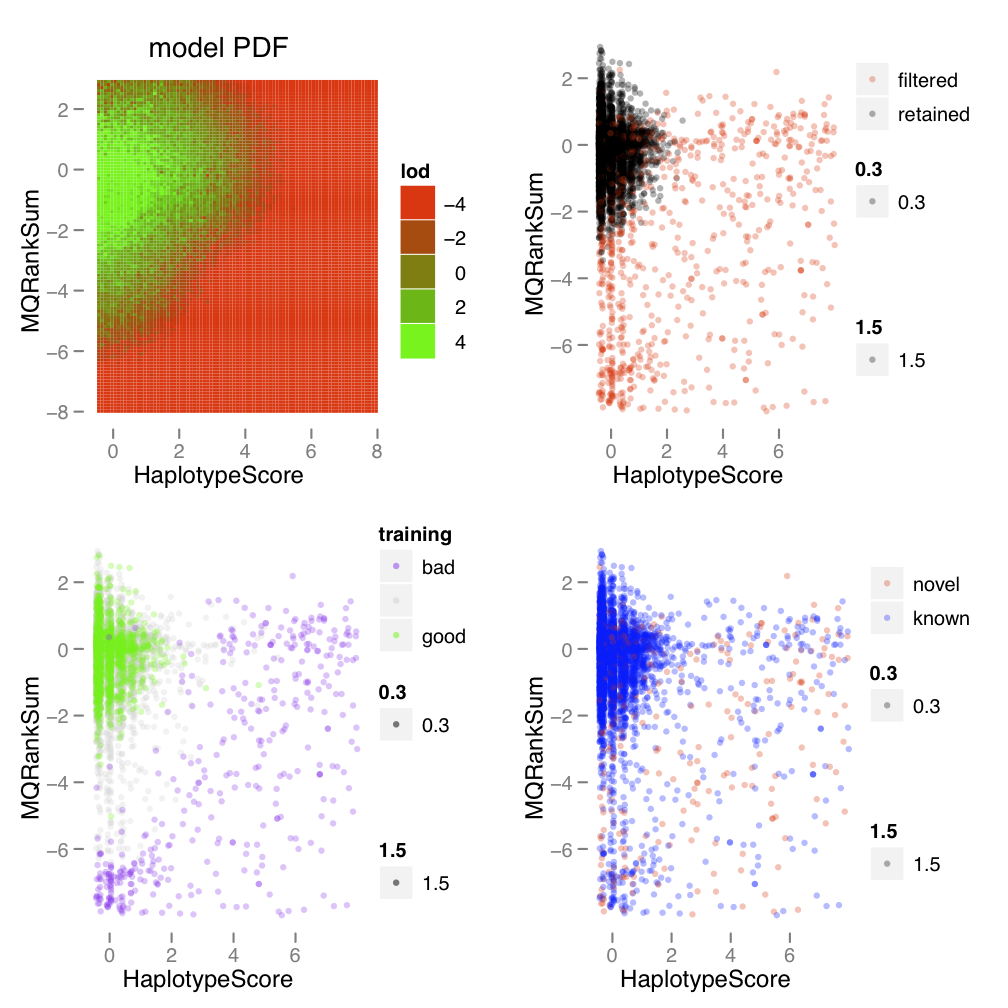
| The variant recalibration step fits a Gaussian mixture model to the contextual annotations given to each variant. By fitting this probability model to the training variants (variants considered to be true-positives), a probability can be assigned to the putative novel variants (some of which will be true-positives, some of which will be false-positives). It is useful for users to see how the probability model was fit to their data. Therefore a modeling report is automatically generated each time VariantRecalibrator is run. For every pairwise combination of annotations used in modeling, a 2D projection of the Gaussian mixture model is shown. | 变体重新校准步骤将高斯混合模型与给每个变体的上下文注释相适应。 通过对训练变体(被认为是真阳性的变体)拟合这个概率模型,可以为假定的新变体分配一个概率(其中一些是真阳性,一些是假阳性) 用户可以看到概率模型是如何与他们的数据相适应的,这是非常有用的。因此,每次运行VariantRecalibrator时都会自动生成一份建模报告。对于建模中使用的每一对注释组合,都会显示高斯混合模型的二维投影。 |
|---|---|
 |
|
| The figure shows one page of an example Gaussian mixture model report that is automatically generated by the VQSR from an example HiSeq call set of SNPs. This page shows the 2D projection of Mapping Quality Rank Sum Test (MQRankSum) versus Haplotype Score (HS) by marginalizing over the other annotation dimensions in the model. | 图中显示了高斯混合模型报告的一个页面,该报告是由VQSR从一个SNP的HiSeq调用集的例子中自动生成的。这一页显示了通过对模型中其他注释维度进行边际化处理,映射质量等级总和检验(MQRankSum)与单倍型分数(HS)的二维投影。 |
| :::info |
Note that this is an old example that uses an annotation, Haplotype Score, that has been deprecated and is no longer available. However, all the points made in the description are still valid.
:::
| 请注意,这是一个旧的例子,它使用的注释,即单倍型得分,已经被废弃,不再可用。然而,描述中的所有观点仍然有效。 |
| In each page there are four panels which show different ways of looking at the 2D projection of the model. The upper left panel shows the probability density function that was fit to the data. The 2D projection was created by marginalizing over the other annotation dimensions in the model via random sampling. Green areas show locations in the space that are indicative of being high quality while red areas show the lowest probability areas. In general putative SNPs that fall in the red regions will be filtered out of the recalibrated call set. | 在每一页中,有四个面板,显示了观察模型的二维投影的不同方式。左上角的面板显示了与数据拟合的概率密度函数。
二维投影是通过随机抽样对模型中的其他注释维度进行边际化处理而产生的。
绿色区域显示空间中表明高质量的位置,而红色区域显示最低概率区域。
一般来说,落在红色区域的假定SNPs将被从重新校准的调用集中过滤掉。 |
| The remaining three panels give scatter plots in which each SNP is plotted in the two annotation dimensions as points in a point cloud. The scale for each dimension is in normalized units. The data for the three panels is the same but the points are colored in different ways to highlight different aspects of the data. In the upper right panel SNPs are colored black and red to show which SNPs are retained and filtered, respectively, by applying the VQSR procedure. The red SNPs didn’t meet the given truth sensitivity threshold and so are filtered out of the call set. The lower left panel colors SNPs green, grey, and purple to give a sense of the distribution of the variants used to train the model. The green SNPs are those which were found in the training sets passed into the VariantRecalibrator step, while the purple SNPs are those which were found to be furthest away from the learned Gaussians and thus given the lowest probability of being true. Finally, the lower right panel colors each SNP by their known/novel status with blue being the known SNPs and red being the novel SNPs. Here the idea is to see if the annotation dimensions provide a clear separation between the known SNPs (most of which are true) and the novel SNPs (most of which are false). | 其余三个板块给出了散点图,其中每个SNP在两个注释维度上被绘制成点云中的一个点。
每个维度的比例都是归一化单位。三个板块的数据是相同的,但点的颜色是不同的,以突出数据的不同方面。
在右上角的面板中,SNPs被染成黑色和红色,以显示哪些SNPs被保留和过滤,分别是通过应用VQSR程序。红色的SNP不符合给定的真相敏感度阈值,所以被过滤出了调用集。
左下角的面板将SNP染成绿色、灰色和紫色,以了解用于训练模型的变体的分布情况。绿色的SNP是那些在进入VariantRecalibrator步骤的训练集中发现的SNP,而紫色的SNP是那些被发现离所学的高斯最远的SNP,因此被赋予最低的真实概率。
最后,右下角的面板按已知/新的状态给每个SNP着色,蓝色为已知SNP,红色为新的SNP。这里的想法是看注释维度是否在已知SNP(大部分是真的)和新SNP(大部分是假的)之间提供了一个明确的分离。 |
| An example of good clustering for SNP calls from the tutorial dataset is shown to the right. The plot shows that the training data forms a distinct cluster at low values for each of the two statistics shown. As the SNPs fall off the distribution in either one or both of the dimensions they are assigned a lower probability (that is, move into the red region of the model’s PDF) and are filtered out. This makes sense based on what the annotated statistics mean; for example the higher values for mapping quality bias indicate more evidence of bias between the reference bases and the alternative bases. The model has captured our intuition that this area of the distribution is highly enriched for machine artifacts and putative variants here should be filtered out. | 右边显示的是教程数据集中SNP调用的一个良好聚类的例子。该图显示,训练数据在所显示的两个统计数据的低值处形成了一个明显的聚类。随着SNP在一个或两个维度上的分布下降,它们被赋予较低的概率(即进入模型PDF的红色区域)并被过滤掉。根据注释的统计数据,这是有意义的;例如,映射质量偏差的数值越高,表明参考碱基和替代碱基之间的偏差证据越多。该模型捕捉到了我们的直觉,即分布的这一区域高度富含机器假象,这里的假定变体应该被过滤掉。
|
|
| |
|
| |
4. Tranches and the tranche plot
| The VQSLOD score provides a continuous estimate of the probability that each variant is true, allowing one to partition the call sets into quality tranches. The main purpose of the tranches is to establish thresholds within your data that correspond to certain levels of sensitivity relative to the truth sets. The idea is that with well calibrated variant quality scores, you can generate call sets in which each variant doesn’t have to have a hard answer as to whether it is in or out of the set. If a very high accuracy call set is desired then one can use the highest tranche, but if a larger, more complete call set is a higher priority than one can dip down into lower and lower tranches. These tranches are applied to the output VCF file using the FILTER field. In this way you can choose to use some of the filtered records or only use the PASSing records. | VQSLOD得分提供了对每个变异体是真实的概率的连续估计,允许人们将调用集划分为质量档次。 分段的主要目的是在你的数据中建立阈值,对应于相对于真相集的某些敏感度水平。我们的想法是,通过校准好的变体质量分数,你可以生成呼叫集,其中每个变体不需要对其是否在呼叫集中有一个硬性的答案。 如果需要一个非常高的准确度的呼叫集,那么可以使用最高的档次,但如果一个更大的、更完整的呼叫集是一个更优先的选择,那么可以下调到更低的档次。 这些档次是使用FILTER字段应用于输出的VCF文件的。通过这种方式,你可以选择使用一些过滤的记录,或者只使用通过的记录。 |
|---|---|
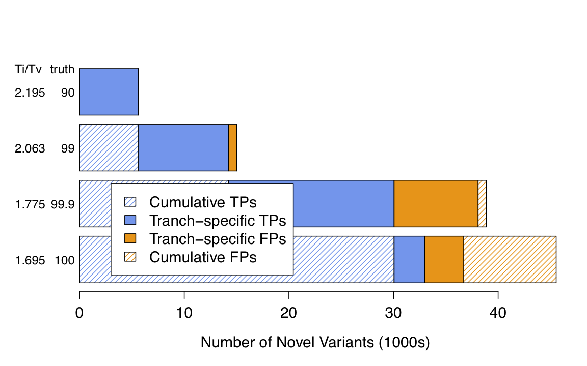
| The first tranche (90 by default, but you can specify your own values) has the lowest value of truth sensitivity but the highest value of novel Ti/Tv; it is extremely specific (almost exclusively real variants in here) but less sensitive (it’s missing a lot). From there, each subsequent tranche introduces additional true positive calls along with a growing number of false positive calls. | 第一个档(默认为90,但你可以指定你自己的值)具有最低的真相灵敏度值,但具有最高的新颖Ti/Tv值;它是非常具体的(这里几乎只有真实的变体),但不太敏感(它缺少很多)。 从这里开始,每一个后续的批次都会引入更多的真阳性呼叫,以及越来越多的假阳性呼叫 |
| A plot of the tranches is automatically generated for SNPs by the VariantRecalibrator tool if you have the requisite R dependencies installed; an example is shown below. | 如果你安装了必要的R依赖,VariantRecalibrator工具会自动生成SNPs的分档图;一个例子显示在下面。 |
 |
|
| This is an example of a tranches plot generated for a HiSeq call set. The x-axis gives the number of novel variants called while the y-axis shows two quality metrics — novel transition to transversion (TiTv) ratio and the overall truth sensitivity. Remember that specificity decreases as the truth sensitivity increases. | 这是一个为HiSeq调用集生成的Tranches图的例子。 X轴给出了被调用的新变体的数量,而Y轴则显示了两个质量指标—新变体与反转体(TiTv)的比率和整体真相灵敏度 请记住,特异性会随着真相灵敏度的增加而降低 |
| The tranches plot is not applicable for indels and will not be generated when the tool is run in INDEL mode. | 转位图不适用于indels,当工具在INDEL模式下运行时,不会产生转位图 |
5. Resource datasets
| This procedure relies heavily on the availability of good resource datasets of the following types: | 这一程序在很大程度上依赖于以下类型的良好资源数据集的可用性: |
|---|---|
Truth resource
| This resource must be a call set that has been validated to a very high degree of confidence. The program will consider that the variants in this resource are representative of true sites (truth=true), and will use them to train the recalibration model (training=true). We will also use these sites later on to choose a threshold for filtering variants based on sensitivity to truth sites. | 这个资源必须是一个已经被验证为非常高置信度的调用集。 该程序将认为该资源中的变体是真实部位的代表(truth=true),并使用它们来训练重新校准模型(training=true)。 我们以后还将使用这些位点,根据对真实位点的敏感性来选择过滤变体的阈值。 |
|---|---|
Training resource
| This resource must be a call set that has been validated to some degree of confidence. The program will consider that the variants in this resource may contain false positives as well as true variants (truth=false), and will use them to train the recalibration model (training=true). | 这个资源必须是一个已经被验证到一定程度的调用集。 该程序将考虑该资源中的变体可能包含假阳性以及真变体(truth=false),并将使用它们来训练重新校准模型(training=true)。 |
|---|---|
Known sites resource
| This resource can be a call set that has not been validated to a high degree of confidence (truth=false). The program will not use the variants in this resource to train the recalibration model (training=false). However, the program will use these to stratify output metrics such as Ti/Tv ratio by whether variants are present in dbsnp or not (known=true). | 该资源可以是一个没有经过高度验证的调用集(true=false)。该程序不会使用该资源中的变体来训练重新校准模型(training=false)。然而,程序将使用这些变体来分层输出指标,如Ti/Tv比率,根据变体是否存在于dbsnp中(已知=true) |
|---|---|
Obtaining appropriate resources
| The human genome training, truth and known resource datasets that are used in our Best Practices workflow applied to human data are all available from our Resource Bundle. | 应用于人类数据的最佳实践工作流程中的人类基因组训练、真相和已知资源数据集都可以从我们的资源包中获得。 |
|---|---|
| If you are working with non-human genomes, you will need to find or generate at least truth and training resource datasets with properties as described above. You’ll also need to assign your set a prior likelihood that reflects your confidence in how reliable it is as a truth set. We recommend Q10 as a starting value, which you can then experiment with to find the most appropriate value empirically. There are many possible avenues of research here. Hopefully the model reporting plots that are generated by the recalibration tools will help facilitate this experimentation. | 如果你正在处理非人类基因组,你将需要至少找到或生成具有上述属性的真相和训练资源数据集。 你还需要给你的数据集分配一个先验可能性,反映你对它作为真相集的可靠性的信心。 我们建议将Q10作为一个起始值,然后你可以通过实验来找到最合适的经验值。这里有许多可能的研究途径。 希望由重新校准工具生成的模型报告图能够帮助促进这种实验 |
6. Problems
| VariantRecalibrator is like a teenager, frequently moody and uncommunicative. There are many things that can put this tool in a bad mood and cause it to fail. When that happens, it rarely provides a useful error message. We’re very sorry about that and we’re working hard on developing a new tool (based on deep learning) that will be more stable and user-friendly. In the meantime though, here are a few things to watch out for. | VariantRecalibrator就像一个青少年,经常喜怒无常,不善于沟通。有很多事情可以让这个工具心情不好,导致它失败。 当这种情况发生时,它很少提供一个有用的错误信息。我们对此非常抱歉,我们正在努力开发一个新的工具(基于深度学习),它将更加稳定和用户友好。 不过,与此同时,这里有一些需要注意的事情。 |
|---|---|
Greedy for data
| This tool expects large numbers of variant sites in order to achieve decent modeling with the Gaussian mixture model. It’s difficult to put a hard number on mimimum requirements because it depends a lot on the quality of the data (clean, well-behaved data requires fewer sites because the clustering tends to be less noisy), but empirically we find that in humans, the procedure tends to work well enough with at least one whole genome or 30 exomes. Anything smaller than that scale is likely to run into difficulties, especially for the indel recalibration. | 这个工具希望有大量的变异位点,以便用高斯混合模型实现合适的建模。 很难给最低要求一个硬性数字,因为它在很大程度上取决于数据的质量(干净的、表现良好的数据需要较少的位点,因为聚类的噪声较小),但根据经验,我们发现在人类中,该程序倾向于在至少一个全基因组或30个外显子中工作得足够好。 任何小于这个规模的东西都有可能遇到困难,特别是对于缩减基因的重新校准。 |
|---|---|
| If you don’t have enough of your own samples, consider using publicly available data (e.g. exome bams from the 1000 Genomes Project) to “pad” your cohort. Be aware however that you cannot simply merge in someone else’s variant calls. You must joint-call variants from the original BAMs with your own samples. We recommend using the GVCF workflow to generate GVCFs from the original BAMs, and joint-call those GVCFs along with your own samples’ GVCFs using GenotypeGVCFs. | 如果你没有足够的自己的样本,可以考虑使用公开的数据(例如来自1000基因组计划的外显子组bams)来 “填充 “你的队列。 但是要注意,你不能简单地合并别人的变体调用。 你必须将原始BAMs中的变异体与你自己的样本联合调用。我们建议使用GVCF工作流程,从原始BAMs中生成GVCF,然后使用GenotypeGVCFs联合调用这些GVCF和你自己样本的GVCF。 |
One other thing that can help is to turn down the number of Gaussians used during training. This can be accomplished by adding --maxGaussians 4 to your command line. This controls the maximum number of different “clusters” (=Gaussians) of variants the program is allowed to try to identify. Lowering this number forces the program to group variants into a smaller number of clusters, which means there will be more variants in each cluster — hopefully enough to satisfy the statistical requirements. Of course, this decreases the level of discrimination that you can achieve between variant profiles/error modes. It’s all about trade-offs; and unfortunately if you don’t have a lot of variants you can’t afford to be very demanding in terms of resolution. |
还有一件事可以帮助你,就是在训练过程中减少高斯的数量。这可以通过在你的命令行中添加—maxGaussians 4来实现。 这可以控制程序被允许尝试识别的不同 “集群”(=高斯)变体的最大数量。 降低这个数字会迫使程序将变异体归入较少的集群,这意味着每个集群中会有更多的变异体—希望能满足统计要求。 当然,这降低了你在变异体特征/错误模式之间所能达到的区分水平。这都是权衡利弊的问题; 不幸的是,如果你没有大量的变体,你就不能在分辨率方面有很高的要求。 |
Annotations are tricky
| VariantRecalibrator assumes that the distribution of annotation values is gaussianly distributed, but we know this assumption breaks down for some annotations. For example, mapping quality has a very different distribution because it is not a calibrated statistic, so in some cases it can destabilize the model. When you run into trouble, excluding MQ from the list of annotations can be helpful. | VariantRecalibrator假设注释值的分布是高斯分布的,但是我们知道这个假设对于某些注释来说是失效的。 例如,mapping质量有一个非常不同的分布,因为它不是一个校准的统计量,所以在某些情况下它会破坏模型的稳定性。当你遇到麻烦时,将MQ从注释列表中排除可能会有帮助 |
|---|---|
| In addition, some of the annotations included in our standard VQSR recommendations might not be the best for your particular dataset. In particular, the following caveats apply: - Depth of coverage (the DP annotation invoked by Coverage) should not be used when working with exome datasets since there is extreme variation in the depth to which targets are captured. In whole genome experiments this variation is indicative of error but that is not the case in capture experiments. - InbreedingCoeff* is a population level statistic that requires at least 10 samples in order to be computed. For projects with fewer samples, or that includes many closely related samples (such as a family) please omit this annotation from the command line. |
此外,我们的标准VQSR建议中包含的一些注释可能不是最适合你的特定数据集。特别是,以下注意事项适用: - 覆盖深度(由Coverage调用的DP注释)在处理外显子组数据集时不应该使用,因为捕获目标的深度有极大的差异。在全基因组实验中,这种变化表明有误差,但在捕获实验中却不是这样的。 - 近亲繁殖系数*是一个群体水平的统计,需要至少10个样本才能计算。对于样本较少的项目,或者包括许多密切相关的样本(如一个家族),请从命令行中省略这一注释。 |
Dependencies
| Plot generation depends on having Rscript accessible in your environment path. Rscript is the command line version of R that allows execution of R scripts from the command line. We also make use of the ggplot2 library so please be sure to install that package as well. See the Common Problems section of the Guide for more details. | 图案的生成取决于你的环境路径中是否有Rscript可以访问 Rscript是R的命令行版本,允许从命令行执行R脚本。我们还使用了 ggplot2 库,所以请确保也安装该软件包 更多细节请参见本指南的常见问题部分 |
|---|---|
Which training sets arguments should I use for running VQSR?
| This document describes the resource datasets and arguments that we recommend for use in the two steps of VQSR (i.e. the successive application of VariantRecalibrator and ApplyRecalibration), based on our work with human genomes, to comply with the GATK Best Practices. The recommendations detailed in this document take precedence over any others you may see elsewhere in our documentation (e.g. in Tutorial articles, which are only meant to illustrate usage, or in past presentations, which may be out of date). | 本文档描述了我们推荐在VQSR的两个步骤(即连续应用VariantRecalibrator和ApplyRecalibration)中使用的资源数据集和参数,这是基于我们在人类基因组方面的工作,以符合GATK最佳实践。 本文件中详述的建议优先于你在我们的文档中可能看到的任何其他建议(例如,在教程文章中,这只是为了说明用法,或者在过去的演讲中,这可能已经过时了) |
|---|---|
| The document covers: - Explanation of resource datasets - Important notes about annotations - Important notes about exome experiments - Argument recommendations for VariantRecalibrator - Argument recommendations for ApplyRecalibration - These recommendations are valid for use with calls generated by both the UnifiedGenotyper and HaplotypeCaller. In the past we made a distinction in how we processed the calls from these two callers, but now we treat them the same way. These recommendations will probably not work properly on calls generated by other (non-GATK) callers. |
Note that VQSR must be run twice in succession in order to build a separate error model for SNPs and INDELs (see the VQSR documentation for more details). | 该文件涵盖:
- 资源数据集的解释
- 关于注释的重要说明
- 关于外显子实验的重要说明
- VariantRecalibrator的参数建议
- ApplyRecalibration的参数建议
- 这些建议对UnifiedGenotyper和HaplotypeCaller产生的调用都是有效的。在过去,我们在处理来自这两个调用器的调用时做了区分,但现在我们以同样的方式对待它们。这些建议对其他(非GATK)调用者产生的调用可能无法正常工作。
请注意,VQSR必须连续运行两次,以便为SNP和INDELs建立单独的错误模型(更多细节见VQSR文档) |
Explanation of resource datasets
| The human genome training, truth and known resource datasets mentioned in this document are all available from our resource bundle. | 本文中提到的人类基因组训练、真相和已知资源数据集都可以从我们的资源包中获得。 |
|---|---|
| If you are working with non-human genomes, you will need to find or generate at least truth and training resource datasets with properties corresponding to those described below. To generate your own resource set, one idea is to first do an initial round of SNP calling and only use those SNPs which have the highest quality scores. These sites which have the most confidence are probably real and could be used as truth data to help disambiguate the rest of the variants in the call set. Another idea is to try using several SNP callers in addition to the UnifiedGenotyper or HaplotypeCaller, and use those sites which are concordant between the different methods as truth data. In either case, you’ll need to assign your set a prior likelihood that reflects your confidence in how reliable it is as a truth set. We recommend Q10 as a starting value, which you can then experiment with to find the most appropriate value empirically. There are many possible avenues of research here. Hopefully the model reporting plots that are generated by the recalibration tools will help facilitate this experimentation. | 如果你正在处理非人类基因组,你将需要至少找到或生成具有与下面描述的属性相对应的真相和训练资源数据集。为了生成你自己的资源集, 一个想法是首先做一个初始的SNP调用,只使用那些具有最高质量分数的SNP。这些具有最高置信度的位点可能是真实的,可以作为真实数据来帮助区分调用集中的其他变体。 另一个想法是,除了UnifiedGenotyper或HaplotypeCaller之外,尝试使用几个SNP调用器,并使用那些在不同方法之间一致的站点作为真实数据。 在这两种情况下,你都需要给你的数据集分配一个先验可能性,以反映你对它作为真相数据的可靠性的信心。我们建议将Q10作为一个起始值,然后你可以通过实验来找到最合适的经验值。 这里有许多可能的研究途径。希望由重新校准工具生成的模型报告图能够帮助促进这种实验。 |
Resources for SNPs
|
- True sites training resource: HapMap - This resource is a SNP call set that has been validated to a very high degree of confidence. The program will consider that the variants in this resource are representative of true sites (truth=true), and will use them to train the recalibration model (training=true). We will also use these sites later on to choose a threshold for filtering variants based on sensitivity to truth sites. The prior likelihood we assign to these variants is Q15 (96.84%).
|
- 真实位点训练资源:HapMap - 该资源是一个SNP调用集,已被验证为非常高的置信度。
该程序将认为该资源中的变体是真实位点的代表(truth=true),并将使用它们来训练重新校准模型(training=true)。
我们以后还将使用这些位点,根据对真实位点的敏感性,选择过滤变体的阈值。我们分配给这些变体的先验可能性是Q15(96.84%)。 |
| —- | —- |
|
- True sites training resource: Omni - This resource is a set of polymorphic SNP sites produced by the Omni geno- typing array. The program will consider that the variants in this resource are representative of true sites (truth=true), and will use them to train the recalibration model (training=true). The prior likelihood we assign to these variants is Q12 (93.69%).
|
- 真实位点训练资源:Omni - 该资源是由Omni基因分型阵列产生的一组多态SNP位点。
该程序将认为该资源中的变体是真实位点的代表(truth=true),并将使用它们来训练重新校准模型(training=true)
我们分配给这些变体的先验可能性是Q12(93.69%)。 |
|
- Non-true sites training resource: 1000G - This resource is a set of high-confidence SNP sites produced by the 1000 Genomes Project. The program will consider that the variants in this re- source may contain true variants as well as false positives (truth=false), and will use them to train the recalibration model (training=true). The prior likelihood we assign to these variants is Q10 (90%).
|
- 非真实位点训练资源:1000G - 该资源是由1000基因组计划产生的一组高置信度SNP位点。
该程序将考虑这个再资源中的变体可能包含真正的变体以及假阳性(truth=false),并将使用它们来训练重新校准模型(training=true)
我们为这些变体分配的先验可能性是Q10(90%)。 |
|
- Known sites resource, not used in training: dbSNP - This resource is a call set that has not been validated to a high degree of confidence (truth=false). The program will not use the variants in this resource to train the recalibration model (training=false). However, the program will use these to stratify output metrics such as Ti/Tv ratio by whether variants are present in dbsnp or not (known=true). The prior likelihood we assign to these variants is Q2 (36.90%).
|
- 已知位点资源,不用于训练:dbSNP—该资源是一个未被验证为高置信度的调用集(true=false)
该程序将不使用该资源中的变体来训练重新校准模型(training=false)。
然而,程序将使用这些变体来分层输出指标,如Ti/Tv比率,以确定变体是否存在于dbsnp中(已知=真)我们分配给这些变体的先验可能性是Q2(36.90%)。 |
Resources for Indels
|
- True sites training resource: Mills - This resource is an indel call set that has been validated to a high degree of confidence. The program will consider that the variants in this resource are representative of true sites (truth=true), and will use them to train the recalibration model (training=true). The prior likelihood we assign to these variants is Q12 (93.69%).
|
- 真正的位点训练集:Mills - 该资源是一个已经被验证为高度可信的indel调用集
该程序将认为该资源中的变体是真实位点的代表(truth=true),并将使用它们来训练重新校准模型(training=true)
我们分配给这些变体的先验可能性是Q12(93.69%)。 |
| —- | —- |
|
- Known sites resource, not used in training: dbSNP - This resource is a call set that has not been validated to a high degree of confidence (truth=false). The program will not use the variants in this resource to train the recalibration model (training=false). However, the program will use these to stratify output metrics such as Ti/Tv ratio by whether variants are present in dbsnp or not (known=true). The prior likelihood we assign to these variants is Q2 (36.90%).
|
- 已知位点资源,不用于训练:dbSNP - 该资源是一个没有经过高度验证的调用集(true=false)
该程序将不使用该资源中的变体来训练重新校准模型(training=false)
然而,程序将使用这些变体来分层输出指标,如Ti/Tv比率,以确定变体是否存在于dbsnp中(已知=真)。我们分配给这些变体的先验可能性是Q2(36.90%)。 |
|
- Non-true sites training resource: Axiom (1000G) - This resource is an indel callset based on the Affymetrix Axiom array on 1000 Genomes Project samples. VQSR will consider that the variants in this resource may contain true variants as well as false positives (truth=false). It will use them to train the recalibration model (training=true). The prior likelihood we assign to these variants is Q10 (90%).
|
- 非真实站点的训练资源:Axiom(1000G)—该资源是基于Affymetrix Axiom阵列对1000个基因组项目样本的indel调用集。
VQSR将考虑该资源中的变体可能包含真实变体以及假阳性(truth=false)
它将使用它们来训练重新校准模型(training=true)。我们分配给这些变体的先验可能性是Q10(90%)。 |
Important notes about annotations
| Some of the annotations included in the recommendations given below might not be the best for your particular dataset. In particular, the following caveats apply: - Depth of coverage (the DP annotation) should not be used when working with exome datasets since there is extreme variation in the depth to which targets are captured! In whole genome experiments this variation is indicative of error but that is not the case in capture experiments. - You may have seen HaplotypeScore mentioned in older documents. That is a statistic produced by UnifiedGenotyper that should only be used if you called your variants with UG. This statistic isn’t produced by the HaplotypeCaller because that mathematics is already built into the likelihood function itself when calling full haplotypes with HC. - The InbreedingCoeff is a population level statistic that requires at least 10 samples in order to be computed. For projects with fewer samples, or that includes many closely related samples (such as a family) please omit this annotation from the command line. |
下面给出的建议中包括的一些注释可能不是对你的特定数据集最好的注释。特别是,以下注意事项适用。 - 覆盖深度(DP注释)在处理外显子组数据集时不应该使用,因为目标被捕获的深度有极大的差异!在全基因组实验中,这种差异表明了错误,但这并不意味着它不存在。在全基因组实验中,这种变化表明了错误,但在捕获实验中却并非如此 - 你可能在以前的文件中提到过HaplotypeScore。这是一个由UnifiedGenotyper产生的统计数字,只有当你用UG调用你的变体时才可以使用。这个统计数字不是由HaplotypeCaller产生的,因为当用HC调用完整的单倍型时,这个数学运算已经内置于似然函数本身。 - 近亲繁殖系数(InbreedingCoeff)是一个群体水平的统计数字,需要至少10个样本才能计算出来。对于样本较少的项目,或者包括许多密切相关的样本(如一个家族),请从命令行中省略这一注释。 |
|---|---|
Important notes for exome capture experiments
| In our testing we’ve found that in order to achieve the best exome results one needs to use an exome SNP and/or indel callset with at least 30 samples. For users with experiments containing fewer exome samples there are several options to explore:
- Add additional samples for variant calling, either by sequencing additional samples or using publicly available exome bams from the 1000 Genomes Project (this option is used by the Broad exome production pipeline). Be aware that you cannot simply add VCFs from the 1000 Genomes Project. You must either call variants from the original BAMs jointly with your own samples, or (better) use the reference model workflow to generate GVCFs from the original BAMs, and perform joint genotyping on those GVCFs along with your own samples’ GVCFs with GenotypeGVCFs.
- You can also try using the VQSR with the smaller variant callset, but experiment with argument settings (try adding ‘—maxGaussians 4’ to your command line, for example). You should only do this if you are working with a non-model organism for which there are no available genomes or exomes that you can use to supplement your own cohort.
| 在我们的测试中,我们发现,为了获得最好的外显子组结果,需要使用至少有30个样本的外显子组SNP和/或indel调用集。对于实验中包含较少外显子组样本的用户来说,有几个选项可以探索:
- 添加额外的样本进行变异调用,可以通过对额外的样本进行测序或使用来自1000基因组项目的公开可用的外显子组bams(Broad外显子组生产流水线使用此选项)
请注意,你不能简单地从1000基因组项目中添加VCF。
你必须从原始BAMs中与你自己的样本联合调用变体,或者(更好)使用参考模型工作流程从原始BAMs中生成GVCFs,并通过GenotypeGVCFs对这些GVCFs和你自己样本的GVCFs进行联合基因分型。
- 您也可以尝试使用VQSR与较小的变体调用集,但要尝试参数设置(例如,尝试在命令行中加入”—maxGaussians 4”)
只有在处理非模式生物体时,没有可用的基因组或外显子可以用来补充自己的队列时,才应该这样做。 |
| —- | —- |
Argument recommendations for VariantRecalibrator
| The variant quality score recalibrator builds an adaptive error model using known variant sites and then applies this model to estimate the probability that each variant is a true genetic variant or a machine artifact. One major improvement from previous recommended protocols is that hand filters do not need to be applied at any point in the process now. All filtering criteria are learned from the data itself. | 变体质量得分重新校准器利用已知的变体位点建立一个自适应的误差模型,然后应用这个模型来估计每个变体是真正的遗传变体或机器假象的概率。 与以前推荐的协议相比,一个主要的改进是,现在不需要在过程中的任何时候应用手工过滤器。 所有的过滤标准都是从数据本身学来的。 |
|---|---|
Common, base command line for VariantRecalibrator
| This is the first part of the VariantRecalibrator command line, to which you need to add either the SNP-specific recommendations or the indel-specific recommendations given further below. | 这是VariantRecalibrator命令行的第一部分,你需要在其中加入特定SNP的建议或下面给出的特定indel的建议: |
|---|---|
| ```bash |
$ gatk VariantRecalibrator \ -R Homo_sapiens_assembly38.fasta \ -V input.vcf.gz \
| |<a name="e6xoo"></a>### SNP specific recommendations for VariantRecalibrator| For SNPs we use both HapMap v3.3 and the Omni chip array from the 1000 Genomes Project as training data. In addition we take the highest confidence SNPs from the project's callset. These datasets are available in the GATK resource bundle. | 对于SNPs,我们使用HapMap v3.3和1000基因组项目的Omni芯片阵列作为训练数据。<br />此外,我们还从项目的调用集中抽取了置信度最高的SNPs。这些数据集可在GATK资源包中找到。 || --- | --- || ```bash-resource:hapmap,known=false,training=true,truth=true,prior=15.0 hapmap_3.3.b37.vcf \-resource:omni,known=false,training=true,truth=true,prior=12.0 1000G_omni2.5.b37.vcf \-resource:1000G,known=false,training=true,truth=false,prior=10.0 1000G_phase1.snps.high_confidence.b37.vcf \-resource:dbsnp,known=true,training=false,truth=false,prior=2.0 dbsnp_138.b37.vcf \-an QD -an MQ -an MQRankSum -an ReadPosRankSum -an FS -an SOR -an DP -an InbreedingCoeff \-mode SNP \
| |
| Please note that these recommendations are formulated for whole-genome datasets. For exomes, we do not recommend using DP for variant recalibration (see below for details of why). | 请注意,这些建议是针对全基因组数据集制定的。对于外显子,我们不建议使用DP进行变体再校准(详细原因见下文)。 |
| Note also that, for the above to work, the input vcf needs to be annotated with the corresponding values (QD, FS, DP, etc.). If any of these values are somehow missing, then VariantAnnotator needs to be run first so that VariantRecalibration can run properly. | 还要注意的是,为了使上述方法奏效,输入的vcf需要注有相应的值(QD、FS、DP等)
如果这些值有任何缺失,那么就需要先运行VariantAnnotator,以便VariantRecalibration能够正常运行 |
| Also, using the provided sites-only truth data files is important here as parsing the genotypes for VCF files with many samples increases the runtime of the tool significantly. | 另外,使用所提供的仅有位点的真实数据文件在这里很重要,因为解析有许多样本的VCF文件的基因型会大大增加该工具的运行时间。 |
| You may notice that these recommendations no longer include the —numBadVariants argument. That is because we have removed this argument from the tool, as the VariantRecalibrator now determines the number of variants to use for modeling “bad” variants internally based on the data. | 你可能注意到,这些建议不再包括—numBadVariants参数。
这是因为我们已经从工具中删除了这个参数,因为现在VariantRecalibrator会根据数据来决定内部建模 “坏 “变异体的数量。 |
Indel specific recommendations for VariantRecalibrator
| When modeling indels with the VQSR we use a training dataset that was created at the Broad by strictly curating the (Mills, Devine, Genome Research, 2011) dataset as as well as adding in very high confidence indels from the 1000 Genomes Project. This dataset is available in the GATK resource bundle. | 当用VQSR建模时,我们使用了一个训练数据集,该数据集是在Broad通过严格策划(Mills, Devine, Genome Research, 2011)数据集以及加入来自1000基因组项目的非常高置信度的缩略词而创建的。这个数据集可在GATK资源包中找到: |
|---|---|
| ```bash |
—maxGaussians 4 \ -resource:mills,known=false,training=true,truth=true,prior=12.0 Mills_and_1000G_gold_standard.indels.b37.vcf \ -resource:dbsnp,known=true,training=false,truth=false,prior=2.0 dbsnp_138.b37.vcf \ -an QD -an DP -an FS -an SOR -an ReadPosRankSum -an MQRankSum -an InbreedingCoeff \ -mode INDEL \
| || Note that indels use a different set of annotations than SNPs. Most annotations related to mapping quality have been removed since there is a conflation with the length of an indel in a read and the degradation in mapping quality that is assigned to the read by the aligner. This covariation is not necessarily indicative of being an error in the same way that it is for SNPs. | 需要注意的是缩减因子使用的注释与SNP不同。<br />大多数与映射质量有关的注释已被删除,因为读数中的缩略词的长度与对准器分配给读数的映射质量的降低存在着混淆。<br /><br />这种共变并不一定像SNP那样表明是一个错误。 || You may notice that these recommendations no longer include the --numBadVariants argument. That is because we have removed this argument from the tool, as the VariantRecalibrator now determines the number of variants to use for modeling "bad" variants internally based on the data. | 你可能注意到,这些建议不再包括--numBadVariants参数。<br />这是因为我们已经从工具中删除了这个参数,因为VariantRecalibrator现在是根据数据来决定用于模拟 "坏 "变体的内部变体数量。 |<a name="ttWj0"></a>## Argument recommendations for ApplyRecalibration| The power of the VQSR is that it assigns a calibrated probability to every putative mutation in the callset. The user is then able to decide at what point on the theoretical ROC curve their project wants to live. Some projects, for example, are interested in finding every possible mutation and can tolerate a higher false positive rate. On the other hand, some projects want to generate a ranked list of mutations that they are very certain are real and well supported by the underlying data. The VQSR provides the necessary statistical machinery to effectively apply this sensitivity/specificity tradeoff. | || --- | --- || | |<a name="pT0Vg"></a>### SNP specific recommendations for ApplyRecalibration| As previously described, we used HapMap 3.3 and the Omni 2.5M chip as our SNP truth set. We typically seek to achieve 99.5% sensitivity to the accessible truth sites, but this is by no means universally applicable: you will need to experiment to find out what tranche cutoff is right for your data. Generally speaking, projects involving a higher degree of diversity in terms of world populations can expect to achieve a higher truth sensitivity than projects with a smaller scope. | 如前所述,我们使用HapMap 3.3和Omni 2.5M芯片作为我们的SNP真相集。<br />我们通常寻求对可获得的真实点达到99.5%的灵敏度,但这绝不是普遍适用的:你需要通过实验来找出适合你的数据的档位截止点。<br /><br />一般来说,涉及世界人口多样性程度较高的项目可望比范围较小的项目获得更高的真理灵敏度。 || --- | --- || ```bash--ts_filter_level 99.5 \-mode SNP \
| |
Indel specific recommendations for ApplyRecalibration
| For indels we use the Mills / 1000 Genomes indel truth set described above. We typically seek to achieve 99.0% sensitivity to the accessible truth sites, but this is by no means universally applicable: you will need to experiment to find out what tranche cutoff is right for your data. Generally speaking, projects involving a higher degree of diversity in terms of world populations can expect to achieve a higher truth sensitivity than projects with a smaller scope. | 对于缩略词,我们使用上述的Mills/1000基因组缩略词真相集。我们通常寻求对可访问的真值站点达到99.0%的灵敏度,但这绝不是普遍适用的:你需要通过实验来找出适合你的数据的批次截止点。一般来说,涉及世界人口多样性程度较高的项目可望比范围较小的项目获得更高的真理灵敏度。 |
|---|---|
| ```bash |
—ts_filter_level 99.0 \ -mode INDEL \ ``` | |

若有收获,就点个赞吧
0 人点赞
