Factorization machine (FM) is one of the representative algorithms that are used for building content-based recommenders model. The algorithm is powerful in terms of capturing the effects of not just the input features but also their interactions. The algorithm provides better generalization capability and expressiveness compared to other classic algorithms such as SVMs. The most recent research extends the basic FM algorithms by using deep learning techniques, which achieve remarkable improvement in a few practical use cases.
Factorization Machine
FM is an algorithm that uses factorization in prediction tasks with data set of high sparsity. The algorithm was original proposed in [1]. Traditionally, the algorithms such as SVM do not perform well in dealing with highly sparse data that is usually seen in many contemporary problems, e.g., click-through rate prediction, recommendation, etc. FM handles the problem by modeling not just first-order linear components for predicting the label, but also the cross-product of the feature variables in order to capture more generalized correlation between variables and label.
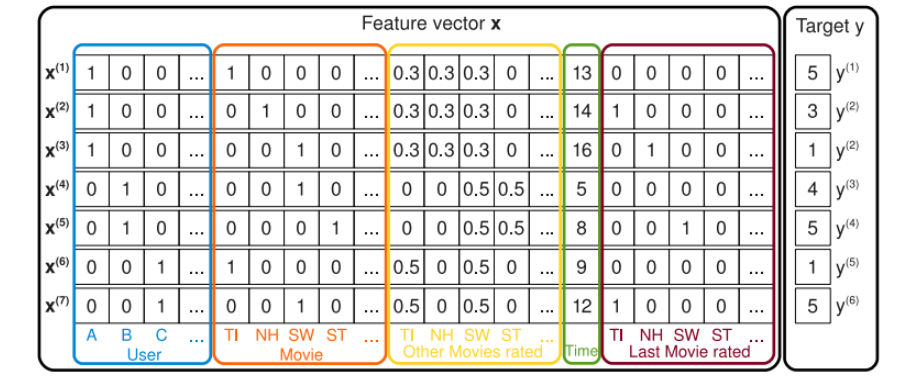
In certain occasions, the data that appears in recommendation problems, such as user, item, and feature vectors, can be encoded into a one-hot representation. Under this arrangement, classical algorithms like linear regression and SVM may suffer from the following problems:
- The feature vectors are highly sparse, and thus it makes it hard to optimize the parameters to fit the model efficienly
- Cross-product of features will be sparse as well, and this in turn, reduces the expressiveness of a model if it is designed to capture the high-order interactions between features
The FM algorithm is designed to tackle the above two problems by factorizing latent vectors that model the low- and high-order components. The general idea of a FM model is expressed in the following equation:
where  and
and  are the target to predict and input feature vectors, respectively.
  is the model parameters for the first-order component.  is the dot product of two latent factors for the second-order interaction of feature variables, and it is defined as:
is the model parameters for the first-order component.  is the dot product of two latent factors for the second-order interaction of feature variables, and it is defined as:
Compared to using fixed parameter for the high-order interaction components, using the factorized vectors increase generalization as well as expressiveness of the model. In addition to this, the computation complexity of the equation (above) is  where
where  and
and  are the dimensionalities of the factorization vector and input feature vector, respectively (see the paper for detailed discussion). In practice, usually a two-way FM model is used, i.e., only the second-order feature interactions are considered to favor computational efficiency.
Proof:

def _build_fm(self):"""Construct the factorization machine part for the model.This is a traditional 2-order FM module.Returns:obj: prediction score made by factorization machine."""with tf.variable_scope("fm_part") as scope:x = tf.SparseTensor(self.iterator.fm_feat_indices,self.iterator.fm_feat_values,self.iterator.fm_feat_shape,)xx = tf.SparseTensor(self.iterator.fm_feat_indices,tf.pow(self.iterator.fm_feat_values, 2),self.iterator.fm_feat_shape,)fm_output = 0.5 * tf.reduce_sum(tf.pow(tf.sparse_tensor_dense_matmul(x, self.embedding), 2)- tf.sparse_tensor_dense_matmul(xx, tf.pow(self.embedding, 2)),1,keep_dims=True,)return fm_output
Field-Aware Factorization Machine
Field-aware factorization machine (FFM) is an extension to FM. It was originally introduced in [2]. The advantage of FFM over FM is that, it uses different factorized latent factors for different groups of features. The “group” is called “field” in the context of FFM. Putting features into fields resolves the issue that the latent factors shared by features that intuitively represent different categories of information may not well generalize the correlation.
Different from the formula for the 2-order cross product as can be seen above in the FM equation, in the FFM settings, the equation changes to:
where  and
and  are the fields of
  and
and  , respectively.
Compared to FM, the computational complexity increases to  . However, since the latent factors in FFM only need to learn the effect within the field, so the values in FFM is usually much smaller than that in FM.
FM/FFM extensions
In the recent years, FM/FFM extensions were proposed to enhance the model performance further. The new algorithms leverage the powerful deep learning neural network to improve the generalization capability of the original FM/FFM algorithms. Representatives of the such algorithms are summarized as below. Some of them are implemented and demonstrated in the microsoft/recommenders repository.
| Algorithm | Notes | References | Example in Microsoft/Recommenders |
|---|---|---|---|
| DeepFM | Combination of FM and DNN where DNN handles high-order interactions | [3] | - |
| xDeepFM | Combination of FM, DNN, and Compressed Interaction Network, for vectorized feature interactions | [4] | notebook / utilities |
| Factorization Machine Supported Neural Network | Use FM user/item weight vectors as input layers for DNN model | [5] | - |
| Product-based Neural Network | An additional product-wise layer between embedding layer and fully connected layer to improve expressiveness of interactions of features across fields | [6] | - |
| Neural Factorization Machines | Improve the factorization part of FM by using stacks of NN layers to improve non-linear expressiveness | [7] | - |
| Wide and deep | Combination of linear model (wide part) and deep neural network model (deep part) for memorisation and generalization | [8] | notebook / utilities |
Implementations
| Implementation | Language | Notes | Examples in Microsoft/Recommenders |
|---|---|---|---|
| libfm | C++ | Implementation of FM algorithm | - |
| libffm | C++ | Original implemenation of FFM algorithm. It is handy in model building, but does not support Python interface | - |
| xlearn | C++ with Python interface | More computationally efficient compared to libffm without loss of modeling effectiveness | notebook |
| Vowpal Wabbit FM | Online library with estimator API | Easy to use by calling API | notebook / utilities |
| microsoft/recommenders xDeepFM | Python | Support flexible interface with different configurations of FM and FM extensions, i.e., LR, FM, and/or CIN | notebook / utilities |
In the FM model building, data is usually represented in the libsvm data format. That is, label feat1:val1 feat2:val2 ..., where label is the target to predict, and val is the value to each feature feat.
FFM algorithm requires data to be represented in the libffm format, where each vector is split into several fields with categorical/numerical features inside. That is, label field1:feat1:val1 field2:feat2:val2 ....
e.g.:
df_feature_original = pd.DataFrame({'rating': [1, 0, 0, 1, 1],'field1': ['xxx1', 'xxx2', 'xxx4', 'xxx4', 'xxx4'],'field2': [3, 4, 5, 6, 7],'field3': [1.0, 2.0, 3.0, 4.0, 5.0],'field4': ['1', '2', '3', '4', '5']})converter = LibffmConverter().fit(df_feature_original, col_rating='rating')df_out = converter.transform(df_feature_original)df_out
| rating | field1 | field2 | field3 | field4 | |
|---|---|---|---|---|---|
| 0 | 1 | 1:1:1 | 2:4:3 | 3:5:1.0 | 4:6:1 |
| 1 | 0 | 1:2:1 | 2:4:4 | 3:5:2.0 | 4:7:1 |
| 2 | 0 | 1:3:1 | 2:4:5 | 3:5:3.0 | 4:8:1 |
| 3 | 1 | 1:3:1 | 2:4:6 | 3:5:4.0 | 4:9:1 |
| 4 | 1 | 1:3:1 | 2:4:7 | 3:5:5.0 | 4:10:1 |

若有收获,就点个赞吧
0 人点赞
