目标检测

为了缓解尺度变化和小目标的问题，现在已经提出了很多方法。

1. 浅层特征与深层特征融合用来检测小目标。
2. dilated/deformable convolution用来增加感受野来提升大目标的检测。
3. 在不同分辨率的层做独立的预测来获取不同的尺度。
4. 上下文用来对模棱两可的情况作分辨。
5. 在一定范围尺度里面训练
6. 在图像金字塔多尺度上推断
7. 预测与NMS融合

目标检测重点

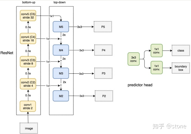
ResNet-FPN

Bottleneck是BasicBlock的升级版，其功能也是构造子网络，resnet18和resnet34中使用了BasicBlock，而resnet50、resnet101、resnet152使用了Bottlenect构造网络。
Bottleneck和BasicBlock网络结构对比如下图所示：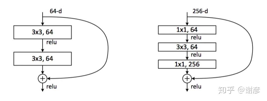

左图中的BasicBlock包含两个3x3的卷积层，右图的Bottleneck包括了三个卷积层，第一个1x1的卷积层用于降维，第二个3x3层用于处理，第三个1x1层用于升维，这样减少了计算量。
https://github.com/pytorch/vision/blob/148bac23afa21ae4df67aeb07a6f0c3bd3b15276/torchvision/models/resnet.py#L30
如果Stride不唯一，shortcut connection分支会有conv_1x1 stride 2的下采样步骤。

stem部分：conv_7x7 stride 2 padding 3 + maxpool 3x3 stride 2 padding 1

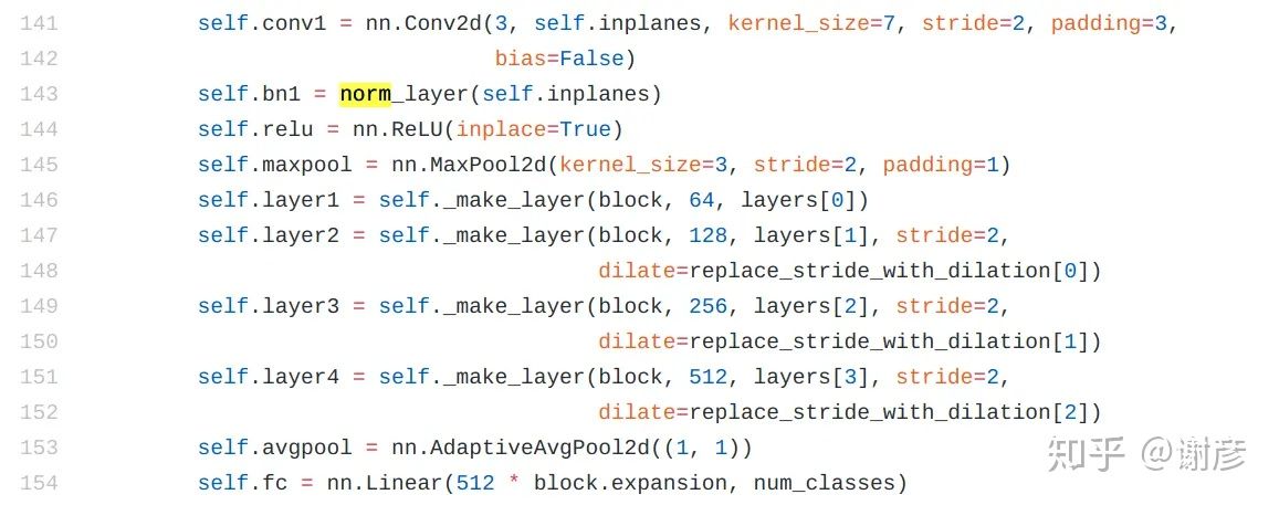
可以看到程序用函数_make_layer创建了四个层，以resnet50为例，各个层中block的个数依次是3,4,6,3个，而每个block（Bottleneck）中又包含三个卷积层，(3+4+6+3)*3共48个卷积层，外加第141行创建的另一卷积层和第154行创建的一个全连接层，总共50个主要层，这也是resnet50中50的含义。

YOLOv3

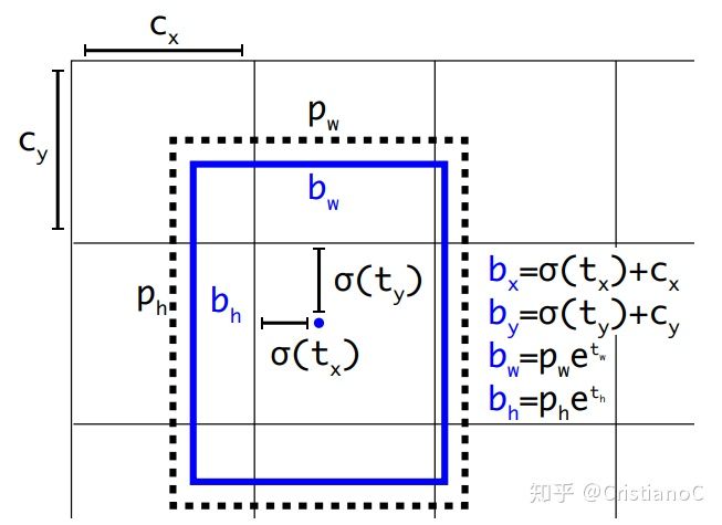
和 分别表示预测框的长宽， 和 分别表示先验框的长和宽。 和 表示的是物体中心距离网格左上角位置的偏移量， 和 则代表网格左上角的坐标。想了解具体详情的读者可以看我解读YOLO v2的那篇文章，也可以看下这面这篇对Yolov3边框预测分析讲解的很好的文章。我们结合代码来看一下（先按照255由来的方式拆解出各个坐标以及位移，再按照公式还原出预测框坐标）：

def decode(self, conv_output, anchors, stride):
        """
        return tensor of shape [batch_size, output_size, output_size, anchor_per_scale, 5 + num_classes]
               contains (x, y, w, h, score, probability)
        stride对应三种feature map的尺寸13,26,52
        anchor_per_scale即为每个cell预测3个bounding box
        """
        conv_shape       = tf.shape(conv_output)
        batch_size       = conv_shape[0]
        output_size      = conv_shape[1]
        anchor_per_scale = len(anchors)
        conv_output = tf.reshape(conv_output, (batch_size, output_size, output_size, anchor_per_scale, 5 + self.num_class))
        conv_raw_dxdy = conv_output[:, :, :, :, 0:2]
        conv_raw_dwdh = conv_output[:, :, :, :, 2:4]
        conv_raw_conf = conv_output[:, :, :, :, 4:5]
        conv_raw_prob = conv_output[:, :, :, :, 5: ]
        #画出（output_size，output_size）的网格
        y = tf.tile(tf.range(output_size, dtype=tf.int32)[:, tf.newaxis], [1, output_size])
        x = tf.tile(tf.range(output_size, dtype=tf.int32)[tf.newaxis, :], [output_size, 1])
        xy_grid = tf.concat([x[:, :, tf.newaxis], y[:, :, tf.newaxis]], axis=-1)
        xy_grid = tf.tile(xy_grid[tf.newaxis, :, :, tf.newaxis, :], [batch_size, 1, 1, anchor_per_scale, 1])
        #要计算位移先把int32转换为float32
        xy_grid = tf.cast(xy_grid, tf.float32)
        #根据公式计算预测框的中心x,y位置
        pred_xy = (tf.sigmoid(conv_raw_dxdy) + xy_grid) * stride
        #根据公式计算预测框的宽高w,h
        pred_wh = (tf.exp(conv_raw_dwdh) * anchors) * stride
        pred_xywh = tf.concat([pred_xy, pred_wh], axis=-1)
        # 根据公式计算含有object的置信度
        pred_conf = tf.sigmoid(conv_raw_conf)
        # 根据公式计算含有类别概率
        pred_prob = tf.sigmoid(conv_raw_prob)
        return tf.concat([pred_xywh, pred_conf, pred_prob], axis=-1)

FCOS

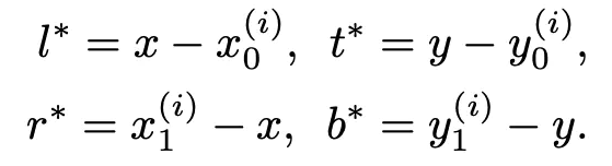
For each location in the feature map, we can map it back onto the input image:

    def _get_points_single(self, featmap_size, stride, dtype, device):
        h, w = featmap_size
        x_range = torch.arange(
            0, w * stride, stride, dtype=dtype, device=device)
        y_range = torch.arange(
            0, h * stride, stride, dtype=dtype, device=device)
        y, x = torch.meshgrid(y_range, x_range)
        points = torch.stack(
            (x.reshape(-1), y.reshape(-1)), dim=-1) + stride // 2
        return points

regress_ranges (tuple[tuple[int, int]]): Regress range of multiple
            level points.
regress_ranges=((-1, 64), (64, 128), (128, 256), (256, 512),
                                 (512, INF)),

Faster-RCNN

def bbox2delta(proposals, gt, means=(0., 0., 0., 0.), stds=(1., 1., 1., 1.)):
    """Compute deltas of proposals w.r.t. gt.
    We usually compute the deltas of x, y, w, h of proposals w.r.t ground
    truth bboxes to get regression target.
    This is the inverse function of `delta2bbox()`
    Args:
        proposals (Tensor): Boxes to be transformed, shape (N, ..., 4)
        gt (Tensor): Gt bboxes to be used as base, shape (N, ..., 4)
        means (Sequence[float]): Denormalizing means for delta coordinates
        stds (Sequence[float]): Denormalizing standard deviation for delta
            coordinates
    Returns:
        Tensor: deltas with shape (N, 4), where columns represent dx, dy,
            dw, dh.
    """
    assert proposals.size() == gt.size()
    proposals = proposals.float()
    gt = gt.float()
    px = (proposals[..., 0] + proposals[..., 2]) * 0.5
    py = (proposals[..., 1] + proposals[..., 3]) * 0.5
    pw = proposals[..., 2] - proposals[..., 0]
    ph = proposals[..., 3] - proposals[..., 1]
    gx = (gt[..., 0] + gt[..., 2]) * 0.5
    gy = (gt[..., 1] + gt[..., 3]) * 0.5
    gw = gt[..., 2] - gt[..., 0]
    gh = gt[..., 3] - gt[..., 1]
    dx = (gx - px) / pw
    dy = (gy - py) / ph
    dw = torch.log(gw / pw)
    dh = torch.log(gh / ph)
    deltas = torch.stack([dx, dy, dw, dh], dim=-1)
    means = deltas.new_tensor(means).unsqueeze(0)
    stds = deltas.new_tensor(stds).unsqueeze(0)
    deltas = deltas.sub_(means).div_(stds)
    return deltas

不同尺度的ROI，使用不同特征层作为ROI pooling层的输入，大尺度ROI就用后面一些的金字塔层，比如P5；小尺度ROI就用前面一点的特征层，比如P4。那怎么判断ROI改用那个层的输出呢？论文的 K 使用如下公式，代码做了一点更改，替换为roi_level：

# 代码里面的计算替换为以下计算方式：
roi_level = min(5, max(2, 4 + log2(sqrt(w * h) / ( 224 / sqrt(image_area)) ) ) )

224是ImageNet的标准输入，k0是基准值，设置为5，代表P5层的输出（原图大小就用P5层），w和h是ROI区域的长和宽，image_area是输入图片的长乘以宽，即输入图片的面积，假设ROI是112 * 112的大小，那么k = k0-1 = 5-1 = 4，意味着该ROI应该使用P4的特征层。k值会做取整处理，防止结果不是整数。