获取更多R语言知识,请关注公众号:医学和生信笔记
医学和生信笔记 公众号主要分享:1.医学小知识、肛肠科小知识;2.R语言和Python相关的数据分析、可视化、机器学习等;3.生物信息学学习资料和自己的学习笔记!
下载
wget -c ftp://ftp.broadinstitute.org/pub/GISTIC2.0/GISTIC_2_0_23.tar.gz
解压
mkdir GISTIC2 # 创建一个目录,用于放下载好的文件mv GISTIC_2_0_23.tar.gz GISTIC2/ && cd GISTIC2/ #把下载好的文件移动过去tar zxf GISTIC_2_0_23.tar.gz # 解压# 此时目录下有这些文件$ lsexamplefiles LICENSE.txtexample_results MATLAB_Compiler_Runtimegistic2 MCR_InstallerGISTIC_2_0_23.tar.gz README.txtGISTICDocumentation_standalone_files refgenefilesGISTICDocumentation_standalone.htm run_gistic_examplegp_gistic2_from_seg sourceINSTALL.txt
安装 Matlab 环境
cd MATLAB_Compiler_Runtime/MCR_Installer/unzip MCRInstaller.zip./install -mode silent -agreeToLicense yes -destinationFolder ~/software/GISTIC2/MATLAB_Compiler_Runtime/ # 改成自己的路径
如果出现 java.lang.InternalError: Can’t connect to X11 window server using ‘:0’ as the value of the DISPLAY variable. 类似的错误,取消显示:unset DISPLAY
安装好之后会出现以下提示,需要你配置环境变量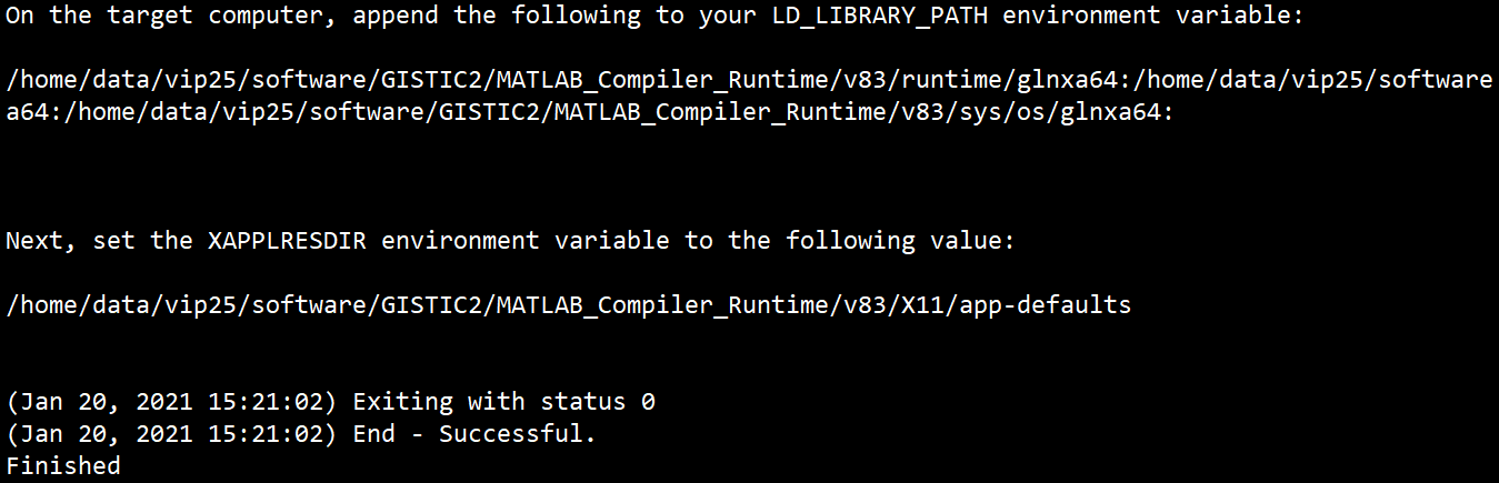
所以接下来我们按照要求设置这些变量。
设置 Matlab 变量
export mcr_root=/home/data/vip25/software/GISTIC2/MATLAB_Compiler_Runtimeexport LD_LIBRARY_PATH=$mcr_root/v83/runtime/glnxa64:$mcr_root/v83/bin/glnxa64:$mcr_root/v83/sys/os/glnxa64:export XAPPLRESDIR=$mcr_root/v83/X11/app-defaults
此时如果不报错就是安装好了
为了使用方便,不用每次运行都需要进入这个文件夹下,需要修改 gistic2 这个东西,首先我们备份一下这个文件,我用的方法比较笨。首先 cat gistic2,然后复制一下出来的东西,然后 vi gistic2_backup,新建一个文件,再把复制的东西粘贴进去。备份好之后再编辑 gistic2 这个文件。
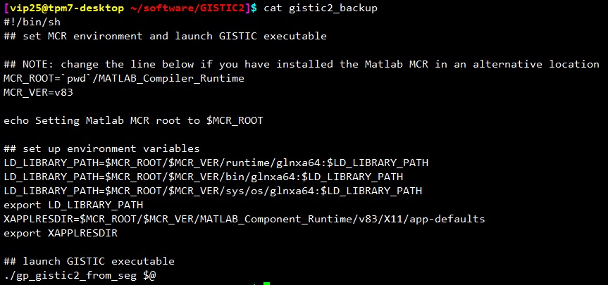
主要就是修改其中的 MCR_ROOT 路径和最后一行 gp_gistic2_from_seg $@ 的路径,做到可以在其他位置调用。
首先看一下目前的位置:
然后更改路径,改成下图所示这样: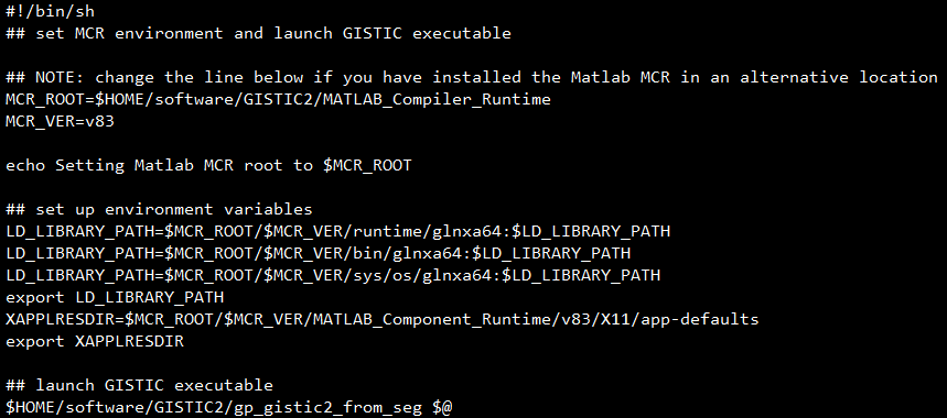
可以看到,除了那 2 个路径的地方外,其余地方都没变,改完之后,就可以在任意位置使用以下代码使用 gistic2 软件了:
## 以后就可以使用这句代码$HOME/software/GISTIC2/gistic2 --helpSetting Matlab MCR root to /home/data/vip25/software/GISTIC2/MATLAB_Compiler_RuntimeGISTIC 2.0 input error:Must supply a base directory.## 看一下常用参数Usage: gp_gistic2_from_seg -b base_dir -seg segmentation_file-refgene ref_gene_file [-mk markers_file] [-alf array_list_file(def:empty)][-cnv cnv_file] [-ta amplifications_threshold(def=.1)] [-td deletions_threshold(def=.1)][-js join_segment_size(def=8)] [-ext extension] [-qvt qv_thresh(def=0.25)][-rx remove_x(def=1)] [-v verbosity_level(def=0)] [-cap cap_val(def=1.5]][-broad run_broad_analysis(def=0)] [-brlen broad_length_cutoff(def=0.98)][-maxseg max_sample_segs(def=2500)] [-res res(def=0.05)] [-conf conf_level(def=0.75)][-genegistic do_gene_gistic(def=0)] [-smalldisk save_disk_space(def=0)][-smallmem use_segarray(def=1)] [-savegene write_gene_files(def=0)][-arb do_arbitration(def=1)] [-twosides use_two_sided(def=0)] [-peaktype peak_types(def=robust)][-saveseg save_seg_data(def=1)] [-savedata write_data_files(def=1)][-armpeel armpeel(def=1)] [-gcm gene_collapse_method(def=mean)][-scent sample_center(def=median)] [-maxspace max_marker_spacing][-logdat islog(def=auto-detect)]
运行 GISTIC 示例文件:
cd .././run_gistic_example
学习下怎么使用 GISTIC2
[vip25@tpm7-desktop ~/software/GISTIC2]$ cat run_gistic_example#!/bin/sh## run example GISTIC analysis## output directoryecho --- creating output directory ---basedir=`pwd`/example_resultsmkdir -p $basedirecho --- running GISTIC ---## input file definitionssegfile=`pwd`/examplefiles/segmentationfile.txtmarkersfile=`pwd`/examplefiles/markersfile.txtrefgenefile=`pwd`/refgenefiles/hg16.matalf=`pwd`/examplefiles/arraylistfile.txtcnvfile=`pwd`/examplefiles/cnvfile.txt## call script that sets MCR environment and calls GISTIC executable./gistic2 -b $basedir -seg $segfile -mk $markersfile -refgene $refgenefile -alf $alf -cnv $cnvfile -genegistic 1 -smallmem 1 -broad 1 -brlen 0.5 -conf 0.90 -armpeel 1 -savegene 1 -gcm extreme
准备自己的文件
根据 GISTICDocumentation_standalone.htm 这个文件里面的提示,我们必须准备的文件只有 2 个:
- segmentationfile.text
- Reference Genome File
但这个软件本身提供了 reference genome file,就在 referencegenefiles 这个文件夹下,并且提供了多个版本:
hg16.mat
hg17.mat
hg18.mat
hg19.mat
hg19.UCSC.addmiR.140312.refgene.mat
hg38.UCSC.add_miR.160920.refgene.mat
所以**真正需要自己准备的只有拷贝数变异文件_**,可以使用 TCGA 官方工具 gdc-client 下载,也可以使用 TCGAbiolinks 包下载(这 2 种方式下载的都是最新的 hg38 版本的,需要和 markersfile 相对应),或者从 firehose下载 hg19 版本的 TCGA 数据。下载后需要整理成和示例文件一样的格式,一共包含 6 列:
The segmentation file contains the segmented data for all the samples identified by GLAD, CBS, or some other segmentation algorithm. (See GLAD file format in the Genepattern file formats documentation.) It is a six column, tab-delimited file with an optional first line identifying the columns. Positions are in base pair units.
The column headers are:
- (1) Sample (sample name)
- (2) Chromosome (chromosome number)
- (3) Start Position (segment start position, in bases)
- (4) End Position (segment end position, in bases)
- (5) Num Markers (number of markers in segment)
(6) Seg.CN (log2() -1 of copy number)
下面是下载和整理的代码:
## cnv segment文件的准备library(dplyr)library(TCGAbiolinks)query <- GDCquery(project = "TCGA-COAD",data.category = "Copy Number Variation",data.type = "Masked Copy Number Segment")GDCdownload(query, method = "api", files.per.chunk = 50)segment_dat <- GDCprepare(query = query)save(segment_dat, file = "COAD_maskedCNVsegment.RData")segment_dat1 <- segment_datsegment_dat1$Sample1 <- substring(segment_dat1$Sample, 1, 16)segment_dat1 <- grep("01A$",segment_dat1$Sample1) %>%segment_dat1[.,]segment_dat1[,1] <- segment_dat1$Samplesegment_dat1 <- segment_dat1[,-c(7:8)]write.table(segment_dat1,"MaskedCopyNumberSegment1.txt",sep="\t",quote = F,col.names = F,row.names = F)
虽然其他文件不用准备,但依然需要学习一下。
markersfile 文件,在这里下载 https://gdc.cancer.gov/about-data/gdc-data-processing/gdc-reference-files。下载如下图中的文件,注意下面的提示,下载下来后需要自己处理,只保留 freqcnv=FALSE 的行。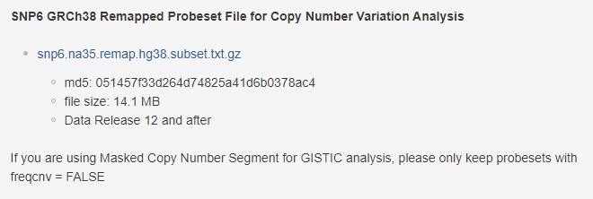
下载完成后先解压,然后读入 R 进行处理,注意自己的路径。下面是代码:## marker files的准备marker <- data.table::fread("./files/snp6.na35.remap.hg38.subset.txt",data.table = F)head(marker)## 查看gistic2.0自带的examplefiles里面的marksfile文件,得知不需要表头,## 只要前三列,并只保存freqcnv == "FALSE"的行marker <- subset(marker, marker$freqcnv == "FALSE")marker <- marker[,1:3]head(marker)write.table(marker, file = "./files/markerfiles.txt", sep = "\t", quote = F, col.names = T, row.names = F)
然后是 CNVfile
There are two options for the file specifying germ line CNVs to be excluded from the analysis. The first option allows CNVs to be identified by marker name and is platform-specific. The second option allows the CNVs to be identified by genomic location, which is platform independent but genome-build dependent.
Option #1: A two column, tab-delimited file with an optional header row. The marker names given in this file must match the marker names given in the markers file. The CNV identifiers are for user use and can be arbitrary. The column headers are:(1) Marker Name
- (2) CNV Identifier
Option #2: A 6 column, tab-delimited file with an optional header row. The ‘CNV Identifier’ is for user use and can be arbitrary. ‘Narrow Region Start’ and ‘Narrow Region End’ are also not used. The column headers are:
- (1) CNV Identifier
- (2) Chromosome
- (3) Narrow Region Start
- (4) Narrow Region End
- (5) Wide Region Start
- (6) Wide Region End
还有一个是 Array List File
The array list file is an optional file identifying the subset of samples to be used in the analysis. It is a one column file with an optional header (array). The sample identifiers listed in the array list file must match the sample names given in the segmentation file.
以上所有文件都是有示例的,需要的可以自己根据示例文件准备。
运行 GISTIC2.0
准备好自己的文件后,就可以进行分析了。
先看下 GDC 官方参数
gistic2 -b <base_directory> -seg <segmentation_file> -mk <marker_file> -refgene <reference_gene_file>-ta 0.1-armpeel 1-brlen 0.7-cap 1.5-conf 0.99-td 0.1-genegistic 1-gcm extreme-js 4-maxseg 2000-qvt 0.25-rx 0-savegene 1(-broad 1)
下面是我的脚本,注意文件路径,需要和 run_gistic_example 在同一个文件夹下:
#!/bin/sh## run GISTIC analysis## output directoryecho --- creating output directory ---basedir=`pwd`/COAD_resultsmkdir -p $basedirecho --- running GISTIC ---## input file definitionssegfile=`pwd`/coadcnvfiles/MaskedCopyNumberSegment1.txtrefgenefile=`pwd`/refgenefiles/hg38.UCSC.add_miR.160920.refgene.mat## call script that sets MCR environment and calls GISTIC executable./gistic2 -b $basedir -seg $segfile -refgene $refgenefile -genegistic 1 -smallmem 1 -broad 1 -brlen 0.5 -conf 0.90 -armpeel 1 -savegene 1 -gcm extreme
输出文件如下: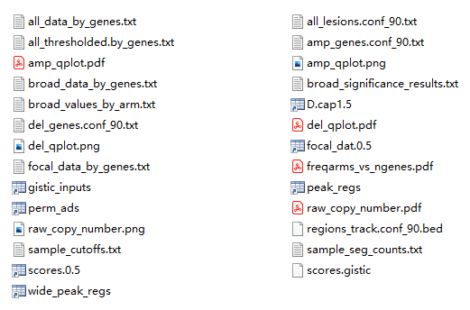
部分结果解释:
- all_data_by_genes.txt —- 基因在不同样本中具体的拷贝数数值
- all_thresholded.by_genes.txt —- 基因在不同样本中拷贝数数值离散化后的结果,-2 代表缺失两个拷 贝,-1 代表缺失一个拷贝,0 代表拷贝数正常,1 代表增加一个拷贝,2 代表扩增两个拷贝
- focal_data_by_genes.txt —- 基因在不同样本中具体的拷贝数数值(只考虑 focal events)
- broad_data_by_genes.txt —- 基因在不同样本中具体的拷贝数数值(只考虑 arm events)
- all_lesions.conf_90.txt —- 识别到的拷贝数扩增和缺失的 Peak 区域
- amp_genes.conf_90.txt —- 识别到的拷贝数扩增的 Peak 区域及区域内涉及到的基因
- del_genes.conf_90.txt —- 识别到的拷贝数缺失的 Peak 区域及区域内涉及到的基因
- broad_significance_results.txt —- 显著发生拷贝数变异的 broad 区域
- broad_values_by_arm.txt —- 染色体臂在样本中的拷贝数数值
- scores.gistic —- 该算法的打分结果,可导入 IGV 进行可视化
结果解读以后再说。。。
待续。。。
获取更多R语言知识,请关注公众号:医学和生信笔记
医学和生信笔记 公众号主要分享:1.医学小知识、肛肠科小知识;2.R语言和Python相关的数据分析、可视化、机器学习等;3.生物信息学学习资料和自己的学习笔记!

若有收获,就点个赞吧
0 人点赞
