liyue 2021/6/30
获取更多R语言知识,请关注公众号:医学和生信笔记
医学和生信笔记 公众号主要分享:1.医学小知识、肛肠科小知识;2.R语言和Python相关的数据分析、可视化、机器学习等;3.生物信息学学习资料和自己的学习笔记!
本次画图使用的数据来自于CIBERSOFT和ssGSEA的结果,需要自己根据给出的格式整理。
画个图
rm(list = ls())library(tidyverse)## -- Attaching packages --------------------------------------- tidyverse 1.3.1 --## v ggplot2 3.3.3 v purrr 0.3.4## v tibble 3.1.1 v dplyr 1.0.6## v tidyr 1.1.3 v stringr 1.4.0## v readr 1.4.0 v forcats 0.5.1## -- Conflicts ------------------------------------------ tidyverse_conflicts() --## x dplyr::filter() masks stats::filter()## x dplyr::lag() masks stats::lag()load(file = "./rdata/coadread_cibersoft.RData")res_cibersort1 <- as.data.frame(res_cibersort,stringsAsFactors = F)knitr::kable(head(res_cibersort1))
| B cells naive | B cells memory | Plasma cells | T cells CD8 | T cells CD4 naive | T cells CD4 memory resting | T cells CD4 memory activated | T cells follicular helper | T cells regulatory (Tregs) | T cells gamma delta | NK cells resting | NK cells activated | Monocytes | Macrophages M0 | Macrophages M1 | Macrophages M2 | Dendritic cells resting | Dendritic cells activated | Mast cells resting | Mast cells activated | Eosinophils | Neutrophils | P-value | Correlation | RMSE | |
|---|---|---|---|---|---|---|---|---|---|---|---|---|---|---|---|---|---|---|---|---|---|---|---|---|---|
| TCGA-AA-3979-01A-01R-1022-07 | 0.0054392 | 0 | 0.0929004 | 0.0000000 | 0 | 0.1345505 | 0.1951179 | 0.0010103 | 0.0059308 | 0.0000000 | 0.0049664 | 0.0000000 | 0.0000000 | 0.2164667 | 0.0475687 | 0.1686659 | 0.0003992 | 0.0043228 | 0.0000000 | 0.0305069 | 0.0000000 | 0.0921542 | 0.4 | 0.0403932 | 1.073114 |
| TCGA-AG-A032-01A-01R-A00A-07 | 0.0896438 | 0 | 0.0584290 | 0.0225665 | 0 | 0.2393689 | 0.0000000 | 0.0785031 | 0.1000758 | 0.0000000 | 0.0000000 | 0.0459226 | 0.0000000 | 0.1619750 | 0.0492802 | 0.0771410 | 0.0356558 | 0.0118161 | 0.0296222 | 0.0000000 | 0.0000000 | 0.0000000 | 0.3 | 0.0451298 | 1.068029 |
| TCGA-AA-3655-01A-02R-1723-07 | 0.0408891 | 0 | 0.0766110 | 0.0228790 | 0 | 0.1981505 | 0.0000000 | 0.0000000 | 0.1043474 | 0.0000000 | 0.0000543 | 0.0000000 | 0.0000000 | 0.2476955 | 0.0859603 | 0.1745513 | 0.0064078 | 0.0114325 | 0.0215842 | 0.0094370 | 0.0000000 | 0.0000000 | 0.1 | 0.1487438 | 1.034526 |
| TCGA-AG-3894-01A-01R-1119-07 | 0.0432472 | 0 | 0.0840875 | 0.0866711 | 0 | 0.1483661 | 0.0396667 | 0.0051174 | 0.0040562 | 0.0000000 | 0.0328460 | 0.0000000 | 0.0019404 | 0.1309107 | 0.0542465 | 0.2809492 | 0.0000000 | 0.0000000 | 0.0493978 | 0.0000000 | 0.0384972 | 0.0000000 | 0.1 | 0.0846817 | 1.047211 |
| TCGA-D5-6535-01A-11R-1723-07 | 0.0411714 | 0 | 0.0791348 | 0.0065910 | 0 | 0.1877118 | 0.0104629 | 0.0620132 | 0.0511255 | 0.0016361 | 0.0245012 | 0.0000000 | 0.0000000 | 0.2825045 | 0.0968499 | 0.1228615 | 0.0000000 | 0.0000000 | 0.0000000 | 0.0334362 | 0.0000000 | 0.0000000 | 0.1 | 0.1516030 | 1.035827 |
| TCGA-CK-4950-01A-01R-1723-07 | 0.0254992 | 0 | 0.1997683 | 0.0966707 | 0 | 0.0985558 | 0.0393477 | 0.0518356 | 0.0388726 | 0.0000000 | 0.0000000 | 0.0000000 | 0.0000000 | 0.1693512 | 0.0402702 | 0.1418299 | 0.0088852 | 0.0000000 | 0.0000000 | 0.0675871 | 0.0022089 | 0.0193177 | 0.1 | 0.1037796 | 1.033874 |
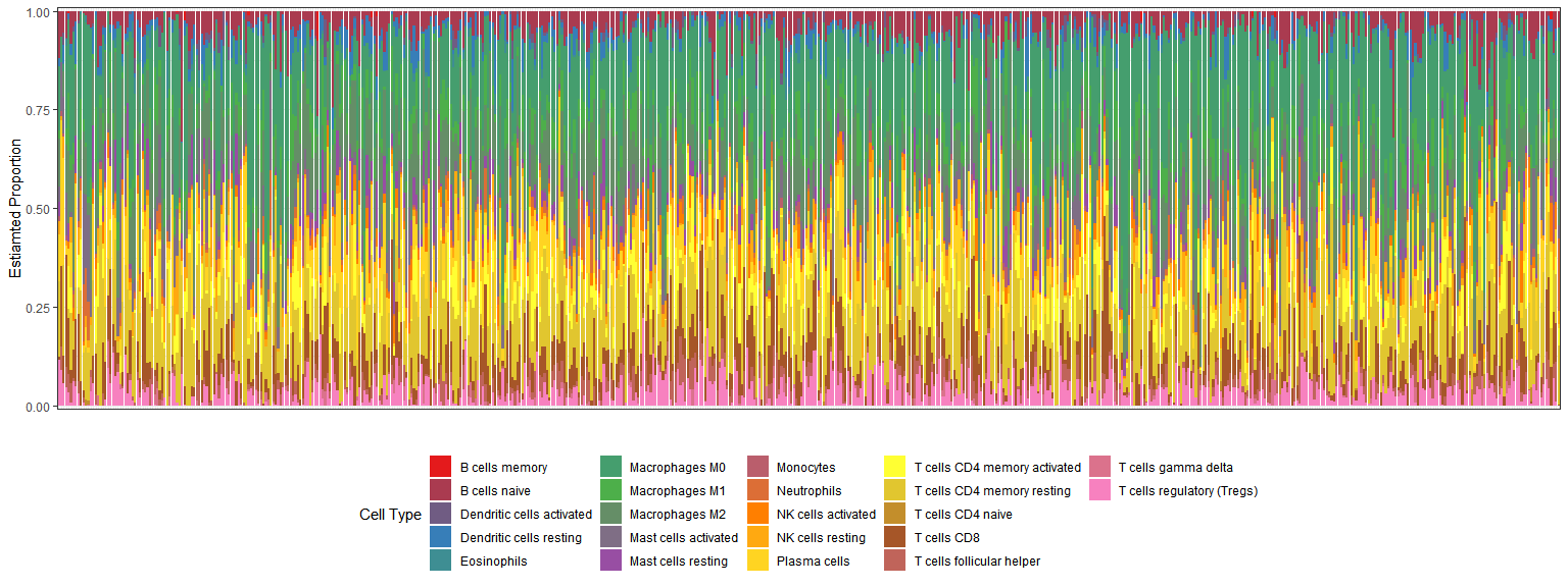
#添加分组信息coread_cibersoft <- res_cibersort1 %>%rownames_to_column(var = "sample_id") %>%mutate(sampletype = ifelse(as.numeric(as.character(str_sub(sample_id,14,15)))<10,"tumor","normal")) %>%select("P-value",Correlation,RMSE,sampletype,everything()) %>%pivot_longer(cols = 6:27,names_to = "celltype",values_to = "proportion")#save(coad_cibersoft,file = "coad_cibersoft.RData")library(ggplot2)library(ggpubr)library(ggsci)#直方图dd1 <- coread_cibersoftlibrary(RColorBrewer)mypalette <- colorRampPalette(brewer.pal(8,"Set1"))ggplot(data =dd1, aes(x = sample_id, y = proportion,fill = celltype))+geom_bar(stat = "identity",position = "stack")+labs(fill = "Cell Type",x = "",y = "Estiamted Proportion") +theme_bw() +theme(axis.text.x = element_blank(),axis.ticks.x = element_blank(),legend.position = "bottom") +scale_y_continuous(expand = c(0.01,0)) +scale_fill_manual(values = mypalette(22))
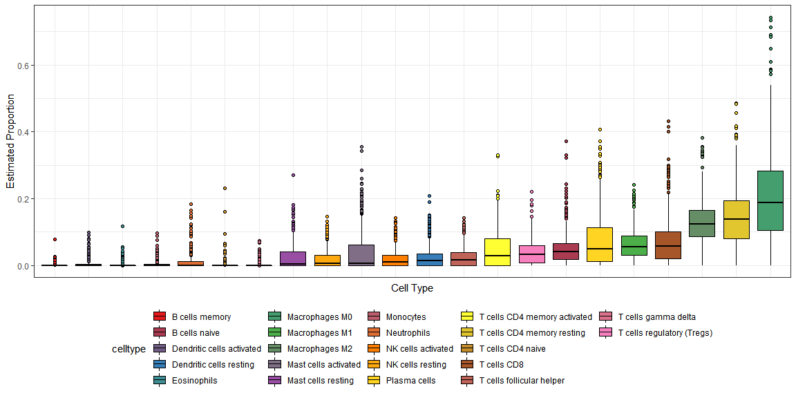
# 有顺序的箱线图library(forcats)ggplot(dd1,aes(fct_reorder(celltype, proportion),proportion,fill = celltype)) +geom_boxplot(outlier.shape = 21,color = "black") +theme_bw() +labs(x = "Cell Type", y = "Estimated Proportion") +theme(axis.text.x = element_blank(),axis.ticks.x = element_blank(),legend.position = "bottom") +scale_fill_manual(values = mypalette(22))
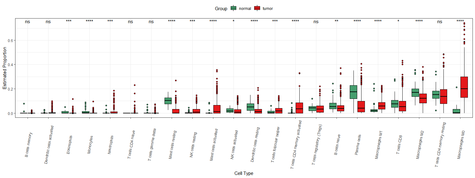
分组箱线图
dd1$Group = ifelse(as.numeric(str_sub(dd1$sample_id,14,15))<10,"tumor","normal")library(ggpubr)ggplot(dd1,aes(fct_reorder(celltype,proportion),proportion,fill = Group)) +geom_boxplot(outlier.shape = 21,color = "black") +theme_bw() +labs(x = "Cell Type", y = "Estimated Proportion") +theme(legend.position = "top") +theme(axis.text.x = element_text(angle=80,vjust = 0.5))+scale_fill_manual(values = mypalette(22)[c(6,1)])+stat_compare_means(aes(group = Group,label = ..p.signif..),method = "kruskal.test")
热图
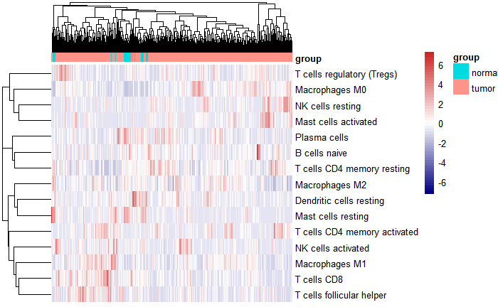
library(pheatmap)k <- apply(res_cibersort1[,-c(23:25)],2,function(x) {sum(x == 0) < nrow(res_cibersort1)/2})table(k)
## k## FALSE TRUE## 7 15
re2 <- as.data.frame(t(res_cibersort1[,-c(23:25)][,k]))Group <- ifelse(as.numeric(as.character(str_sub(rownames(res_cibersort1),14,15)))<10, "tumor","normal")an <- data.frame(group = Group,row.names = rownames(res_cibersort1))pheatmap(re2,scale = "row",show_colnames = F,annotation_col = an,color = colorRampPalette(c("navy", "white", "firebrick3"))(50))
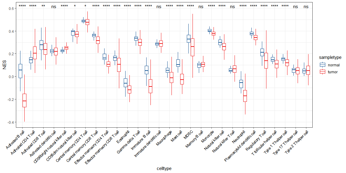
### 画图rm(list = ls())load(file = "./rdata/gsva_data_TCGA_COADREAD.Rdata")coread_gsva <- as.data.frame(t(gsva_data))test <- coread_gsva[1:10,1:10]# 添加分组信息library(tidyverse)coread_gsva <- coread_gsva %>%rownames_to_column(var = "sample_id") %>%mutate(sampletype = ifelse(as.numeric(as.character(str_sub(sample_id,14,15)))<10,"tumor","normal")) %>%select(sampletype,everything())#画图dd1 <- coread_gsva %>%pivot_longer(cols=3:30,names_to= "celltype",values_to = "NES")library(ggplot2)library(ggpubr)library(ggsci)#箱线图,还可以画小提琴图等ggplot(data =dd1, aes(x = celltype, y = NES))+geom_boxplot(aes(color = sampletype),outlier.shape = NA)+scale_color_lancet()+theme_bw()+theme(axis.text.x = element_text(angle = 45, hjust = 1, colour = "black"))+stat_compare_means(aes(group=sampletype), label = "p.signif")
获取更多R语言知识,请关注公众号:医学和生信笔记
医学和生信笔记 公众号主要分享:1.医学小知识、肛肠科小知识;2.R语言和Python相关的数据分析、可视化、机器学习等;3.生物信息学学习资料和自己的学习笔记!

若有收获,就点个赞吧
0 人点赞
