1 第一个文件forward.py
放前向传播的函数,前向传播就是搭建网络结构,设计网络结构。一般需要包含三个函数
# 定义前向传播过程def forward(x,regularizer):w =b =y =return y# 给权重赋初值def get_weight(shape, regularizer):w = tf.Variable(tf.random_normal(shape), dtype=tf.float32)tf.add_to_collection('losses', tf.contrib.layers.l2_regularizer(regularizer)(w))return w# 给偏置赋初值def get_bias(shape):b = tf.Variable(tf.constant(0.01, shape=shape))return b
2 第二个文件backward.py
反向传播就是训练网络,优化网络参数,该文件可以包含损失函数、指数衰减学习率、滑动平均
def backard():x = tf.placeholder()y = tf.placeholder()y = forward.forward(x,REGULARIZER)global_step = tf.Variable(0,trainable =False)loss =## 损失函数#loss第一种是一般求差值的loss,一种是交叉熵的loss,另一种是正则化的loss#loss_mse = tf.reduce_mean(tf.square(y-y_))# 一般loss#loss_ce = tf.reduce_mean(tf.nn.sparse_softmax_cross_entropy_with_logits(logits=y,labels = tf.argmax(y_,1)))# 交叉熵#loss_total = loss_mse + tf.add_n(tf.get_collection('losses'))# 正则化的loss## 指数衰减学习率learning_rate = tf.train.exponential_decay(LEARNING_RATE_BASE,global_step,#数据集总样本数/Batch_sizeLEARNING_RATE_DECAY,staircase =True)#定义反向传播方法train_step = tf.train.AdamOptimizer(0.0001).minimize(loss,global_step =global_step)## 滑动平均ema = tf.train.ExponentialMovingAverage(衰减率MOVING_AVERAGE_DECAY, 当前轮数global_step)#滑动平均ema_op = ema.apply(tf.trainable_variables())#每运行此句,所有待优化的参数求滑动平均# 通常我们把滑动平均与训练过程绑定在一起,使它们合成一个训练节点。如下所示with tf.control_dependencies([train_step,ema_op]):train_op = tf.no_op(name='train')with tf.Session() as sess:init_op = tf.global_variables_initializer()#初始化sess.run(init_op)#初始化STEPS = 3000 # 定义轮数for i in range(STEPS):#三千轮start = (i*BATCH_SIZE) % 32 #8个数据 为一个数据块输出end = (i*BATCH_SIZE) % 32 + BATCH_SIZE #[i:i+8]sess.run(train_step, feed_dict={x: X[start:end], y_: Y[start:end]})#训练if __name__ = '__main__':backward()
3 模块化设计网络举例
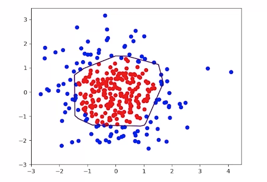
数据X[x0,x1]为正态分布随机点,标注Y当 时y= 1(标记为红色),其余y_=0(标记未蓝色)
(1)生成数据集generateds.by
#coding:utf-8#生成模拟数据集import numpy as npimport matplotlib.pyplot as pltseed = 2def generateds():#基于seed产生随机数rdm = np.random.RandomState(seed)#随机数返回300行2列的矩阵,表示300组坐标点(x0,x1)作为输入数据集X = rdm.randn(300,2)#从X这个300行2列的矩阵中取出一行,判断如果两个坐标的平方和小于2,给Y赋值1,其余赋值0#作为输入数据集的标签(正确答案)Y_ = [int(x0*x0 + x1*x1 <2) for (x0,x1) in X]#遍历Y中的每个元素,1赋值'red'其余赋值'blue',这样可视化显示时人可以直观区分Y_c = [['red' if y else 'blue'] for y in Y_]#对应颜色Y_c#对数据集X和标签Y进行形状整理,第一个元素为-1表示跟随第二列计算,第二个元素表示多少列,可见X为两列,Y为1列X = np.vstack(X).reshape(-1,2)#整理形状Y_ = np.vstack(Y_).reshape(-1,1)#整理形状return X, Y_, Y_c#print X#print Y_#print Y_c#用plt.scatter画出数据集X各行中第0列元素和第1列元素的点即各行的(x0,x1),用各行Y_c对应的值表示颜色(c是color的缩写)#plt.scatter(X[:,0], X[:,1], c=np.squeeze(Y_c))#plt.show()
(2)前向传播 forward.py,设计了神经网络结构
#coding:utf-8#前向传播就是搭建网络import tensorflow as tf#定义神经网络的输入、参数和输出,定义前向传播过程def get_weight(shape, regularizer):#(shape:W的形状,regularizer正则化)w = tf.Variable(tf.random_normal(shape), dtype=tf.float32)#赋初值,正态分布权重tf.add_to_collection('losses', tf.contrib.layers.l2_regularizer(regularizer)(w))#把正则化损失加到总损失losses中return w#返回w#tf.add_to_collection(‘list_name’, element):将元素element添加到列表list_name中def get_bias(shape): #偏执bb = tf.Variable(tf.constant(0.01, shape=shape)) #偏执b=0.01return b#返回值def forward(x, regularizer):#前向传播w1 = get_weight([2,11], regularizer)#设置权重b1 = get_bias([11])#设置偏执y1 = tf.nn.relu(tf.matmul(x, w1) + b1)#计算图w2 = get_weight([11,1], regularizer)#设置权重b2 = get_bias([1])#设置偏执y = tf.matmul(y1, w2) + b2 #计算图return y#返回值
(3)反向传播 backward.py
#coding:utf-8#0导入模块 ,生成模拟数据集import tensorflow as tfimport numpy as npimport matplotlib.pyplot as pltimport opt4_8_generatedsimport opt4_8_forwardSTEPS = 40000BATCH_SIZE = 30LEARNING_RATE_BASE = 0.001LEARNING_RATE_DECAY = 0.999REGULARIZER = 0.01#正则化def backward():#反向传播x = tf.placeholder(tf.float32, shape=(None, 2))#占位y_ = tf.placeholder(tf.float32, shape=(None, 1))#占位#X:300行2列的矩阵。Y_:坐标的平方和小于2,给Y赋值1,其余赋值0X, Y_, Y_c = opt4_8_generateds.generateds()y = opt4_8_forward.forward(x, REGULARIZER)#前向传播计算后求得输出yglobal_step = tf.Variable(0,trainable=False)#轮数计数器#指数衰减学习率learning_rate = tf.train.exponential_decay(LEARNING_RATE_BASE,#学习率global_step,#计数300/BATCH_SIZE,LEARNING_RATE_DECAY,#学习衰减lüstaircase=True)#选择不同的衰减方式#定义损失函数loss_mse = tf.reduce_mean(tf.square(y-y_))#均方误差loss_total = loss_mse + tf.add_n(tf.get_collection('losses'))#正则化#定义反向传播方法:包含正则化train_step = tf.train.AdamOptimizer(learning_rate).minimize(loss_total)with tf.Session() as sess:init_op = tf.global_variables_initializer()#初始化sess.run(init_op)#初始化for i in range(STEPS):start = (i*BATCH_SIZE) % 300end = start + BATCH_SIZE#3000轮sess.run(train_step, feed_dict={x: X[start:end], y_:Y_[start:end]})if i % 2000 == 0:loss_v = sess.run(loss_total, feed_dict={x:X,y_:Y_})print("After %d steps, loss is: %f" %(i, loss_v))xx, yy = np.mgrid[-3:3:.01, -3:3:.01]#网格坐标点grid = np.c_[xx.ravel(), yy.ravel()]probs = sess.run(y, feed_dict={x:grid})probs = probs.reshape(xx.shape)plt.scatter(X[:,0], X[:,1], c=np.squeeze(Y_c)) #画点plt.contour(xx, yy, probs, levels=[.5])#画线plt.show()#显示图像if __name__=='__main__':backward()

若有收获,就点个赞吧
0 人点赞
