1.import os

将图导出保存在文件夹里定义保存图片函数

import numpy as np
import pandas as pd
import os #保存文件包
import matplotlib.pyplot as plt

2.定义保存图片函数:

# 根文件夹
root_dir="."
# 创建目录二级目录多层
model_id="linear_model"
def save_fig(file_name):
#     组装文件目录
    path=os.path.join(root_dir,"images",model_id)
#     判断路径是否存在
    if not os.path.exists(path):
#         不存在就创建path路径
        os.makedirs(path)
#     保存文件创建图片文件名
#     文件地址
    path=os.path.join(path,file_name)
    print("Saving figure",file_name)
    plt.savefig(path,format="png",dpi=300)
    print(path)

3.生成线性数据: θ+θ1x

特征数据和标签数据用随机数生成.

# 随机种子
# np.random.seed(2)
# 生成训练数据(特征部分)
x=2*np.random.rand(100,1)
# 生成训练数据(特标签部分)
y=4+3*x+np.random.randn(100,1)

4.画出模型数据散点图:

参数rotation=0 坐标轴文字翻转
plt.axis([0,2,0,15]) 设置坐标轴范围
保存图片:save_fig(“linera_scatter.png”)

# rotation 翻转文字
plt.scatter(x,y,color="#fff345")#画图
plt.xlabel("$x_1$",fontsize=16)
plt.ylabel("$y$",fontsize=16,rotation=0)
plt.axis([0,2,0,15])
plt.show()
save_fig("linera_scatter.png")

5.建立模型:#从sklearn包里导入线性回归模型

创建线性回归对象: LinearRegression()
拟合训练数据: linreg.fit(x, y)
做预测 :lin_reg.predict(x_new)
输出截距lin_reg.intercept,,斜率 linreg.coef

from sklearn.linear_model import LinearRegression

模型数据测验:

# 创建线性回归对象
lin_reg = LinearRegression() # 调用构造函数  pd.DataFrame()
# 拟合训练数据
lin_reg.fit(x, y)
# 输出截距，斜率
lin_reg.intercept_, lin_reg.coef
#预测测试数据
x_new = np.array([[0], [2]]) # 两行一列的数组
#对测试集进行预测
lin_reg.predict(x_new)

数据80条为训练数据20条为测试数据:
导入分割模块:

from sklearn.model_selection import train_test_split

分割数据块为4部分:

x_train,x_test,y_train,y_test=train_test_split(x,y,test_size=20,random_state=0)

预测三步走:

lin_reg=LinearRegression()
lin_reg.fit(x_train,y_train)
lin_reg.predict(x_test)
对比test集标签
y_test

对模型评分:score

lin_reg.score(x,y)

一.批量梯度下降:

生成俩列特征数据前面填充一列:

x_b = np.hstack((np.ones((100, 1)), x))
x_b

# 步长 step
eta = 0.1
# 迭代次数
n_iterations = 1000
# 数据量
 m = len(x_b)#数据形状
#初始化参数
theta = np.random.randn(2,1)
# 梯度下降公式及参数更新公式
for _ in range(n_iterations):# 限定迭代次数
    gradients = (1/m) * x_b.T.dot(x_b.dot(theta) - y) #梯度求解公式
    theta = theta - eta * gradients #更新theta

# 提供画图的横坐标画图
# 测试集数据
x_new=np.array([[0],[2]])
# 做测试的数据np.c_yu\\与stack一样
x_new_b=np.c_[np.ones((2,1)),x_new]
print(x_new)
print(x_new_b)

函数版:
theta_path_bgd = []
列表收集迭代更新的theta,最后画迭代图

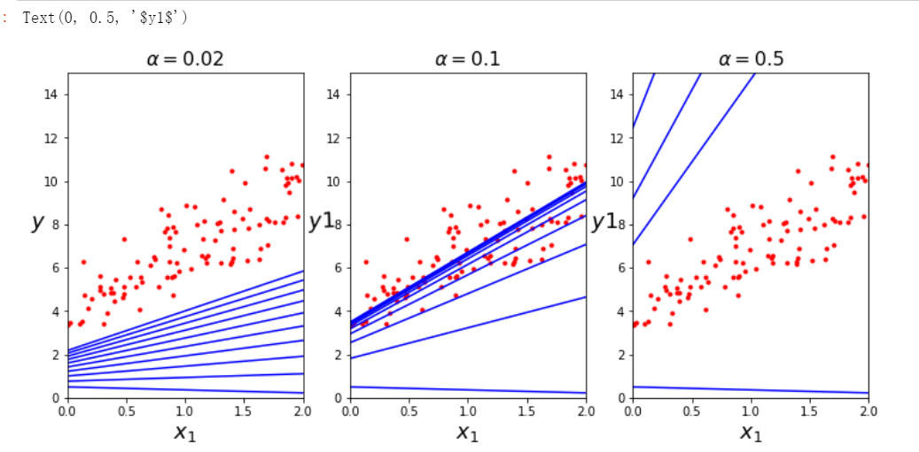
# 为了保存每次更新的theta
theta_path_bgd = []
# [1,2] [2,4]收集θ,最后画三个图
def plot_gradient_descent(theta, eta, theta_path=None,):
    m = len(x_b)#数据形状
    plt.plot(x, y, "r.")#散点图源数据
    n_iterations = 1000 #迭代次数
    for i in range(n_iterations):
        if i < 10:#取前10次
            # 测试集预测的结果
            y_predict = x_new_b.dot(theta) #
            # 测试集确定的直线
            plt.plot(x_new, y_predict, "b-")
        # 使用训练集计算梯度
        gradients = 2/m * x_b.T.dot(x_b.dot(theta) - y)
        # 参数更新公式
        theta = theta - eta * gradients
        if theta_path is not None: #把每个theta添加起来
            theta_path.append(theta)
    plt.xlabel("$x_1$", fontsize=18)
    plt.axis([0, 2, 0, 15])
#     eta 专业步长符号
#     plt.title(r"$\eta = {}$".format(eta), fontsize=16)
    plt.title(r"$\alpha = {}$".format(eta), fontsize=16)

画图:

np.random.seed(42)
theta=np.random.randn(2,1)
fig,ax=plt.subplots(1,3,figsize=(12,5))
plt.subplot(131)
plot_gradient_descent(theta, eta=0.02)
plt.ylabel("$y$",rotation=0,fontsize=18)
plt.subplot(132)
plot_gradient_descent(theta, eta=0.1,theta_path=theta_path_bgd)
plt.ylabel("$y1$",rotation=2,fontsize=18)
plt.subplot(133)
plot_gradient_descent(theta, eta=0.5)
plt.ylabel("$y1$",rotation=0,fontsize=18)

随机梯度下降

theta_path_sgd=[]
m=len(x_b)
np.random.seed(42)

n_epochs参数控制外层循环遍历次数
内层循环取每个数据

n_epochs=2
eta=0.1
theta=np.random.randn(2,1)
plt.plot(x, y, "r.")#散点图源数据
for epoch in range(n_epochs):
    for j in range(m):
        if j<10 and epoch==0:
#             测试集预测y
            y_predict=x_new_b.dot(theta)
             # 测试集确定的直线
            plt.plot(x_new, y_predict, "b-")
        x1=x_b[j:j+1]
        y1=y[j:j+1]
        gradients = 2 * x1.T.dot(x1.dot(theta) - y1)
        theta = theta - eta * gradients
        theta_path_sgd.append(theta)
plt.xlabel("$x_1$", fontsize=18)
plt.axis([0, 2, 0, 15])
#     eta 专业步长符号
plt.title(r"$\alpha = {}$".format(eta), fontsize=16)
# boac
save_fig('sgd_plot')

小批量梯度下降

注意时间

theta_path_mgd = []
n_iterations = 5
minibatch_size = 20#
np.random.seed(42)
theta = np.random.randn(2,1)  # random initialization
for epoch in range(n_iterations):
#     # 数据洗牌,产生一个新的随机顺序
#     shuffled_indices = np.random.permutation(m)
#     x_b_shuffled = x_b[shuffled_indices]
#     y_shuffled = y[shuffled_indices]
    for i in range(0, m, minibatch_size):
        xi = x_b[i:i+minibatch_size]
        yi = y[i:i+minibatch_size]
        gradients = 2/minibatch_size * xi.T.dot(xi.dot(theta) - yi)
        eta = 0.1
        theta = theta - eta * gradients
        theta_path_mgd.append(theta)

将列表数据转化为array

theta_path_bgd = np.array(theta_path_bgd)
theta_path_sgd = np.array(theta_path_sgd)
theta_path_mgd = np.array(theta_path_mgd)

画图:

plt.figure(figsize=(7,4))
plt.plot(theta_path_sgd[:, 0], theta_path_sgd[:, 1], "r-s", linewidth=1, label="Stochastic")
plt.plot(theta_path_mgd[:, 0], theta_path_mgd[:, 1], "g-+", linewidth=2, label="Mini-batch")
plt.plot(theta_path_bgd[:, 0], theta_path_bgd[:, 1], "b-o", linewidth=3, label="Batch")
plt.legend(loc="upper left", fontsize=16)
plt.xlabel(r"$\theta_0$", fontsize=20)
plt.ylabel(r"$\theta_1$   ", fontsize=20, rotation=0)
plt.axis([2.5, 4.5, 2.3, 3.9])
save_fig("gradient_descent_paths_plot")
plt.show()