实验目的
1、了解 python 中的可视化库
2、掌握 python 中 pandas 库、seaborn 库的使用
3、掌握 python 中 bokeh 库、pyqtgraph 库的使用
实验环境
1、64 位电脑,8G 以上内存
2、win10 系统
3、matplotlib 和 pandas、seaborn、bokeh 和 pyqtgraph 库
实验步骤:
1. pandas 库的使用
(1)安装
pip install pandas
(2)Series 的创建与输出
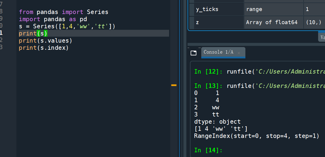
from pandas import Seriesimport pandas as pds = Series([1,4,'ww','tt'])print(s)print(s.values)print(s.index)
(3)自定义索引
列表的索引只能是从 0 开始的整数,Series 数据类型在默认情况下,其索引也是如此。不过,区别于
列表的是 Series 可以自定义以下索引 s2,输出 s2,根据索引修改 s2
from pandas import Seriesimport pandas as pds2 = Series(['wangxing','man',24],index=['name','sex','age'])print(s2)print(s2['name'])s2['name']='zhangsan'print(s2['name'])

(4) 另外一种定义 Series 的方法,观察输出结果
from pandas import Seriesimport pandas as pdsd = {'python':9000,'c++':9001,'c#':9000}s3 = Series(sd)print(s3)

(5) 定义 Series,省略 index
from pandas import Series,DataFramedata = {"name":['google','baidu','yahoo'],"marks":[100,200,300],"price":[1,2,3]}f1 = DataFrame(data)print(f1) #观察输出结果

(6) 定义 Series,加上 index
from pandas import Series,DataFramedata = {"name":['google','baidu','yahoo'],"marks":[100,200,300],"price":[1,2,3]}f1 = DataFrame(data)newdata = {'lang':{'first':'python','second':'java'},'price':{'first':5000,'second':2000}}f4 = DataFrame(newdata)print(f4)print(f4['lang']) #输出某一列print(f4.loc['first']) #输出某一行print(f4['lang']['first']) #输出某个值

(7)练习教材 P203,例 8-19,观察程序输出结果。
8-19
import pandas as pdimport numpy as npimport matplotlib.pyplot as plts = pd.Series(np.random.randn(10).cumsum(), index=np.arange(0, 100, 10))s.plot()plt.show()

(8)练习教材 P205,例 8-20,观察程序输出结果。
8-20
from pandas import DataFrame,Seriesimport pandas as pdimport numpy as npimport matplotlib.pyplot as pltdf = pd.DataFrame(np.random.randn(10, 4).cumsum(0),columns=['A', 'B', 'C', 'D'],index=np.arange(0, 100, 10))df.plot()plt.show()

2. seaborn 库的使用
(1)安装 seaborn
(2)练习 p210 例 8-24
8-24
import numpy as npimport pandas as pdimport matplotlib.pyplot as pltimport seaborn as snssns.set_style("darkgrid")plt.plot(np.arange(10))plt.show()

3. bokeh 库的使用
(1)安装
(2)练习 p215 例 8-28
8-28
from bokeh.plotting import figure, output_file, showoutput_file("patch.html")p = figure(plot_width=400, plot_height=400)p.patch([1, 2, 3, 4, 5], [6, 7, 8, 9, 10], alpha=0.5, line_width=2)show(p)

(3)练习 p216 例 8-29、例 8-30
8-29
from bokeh.plotting import figure, output_file, showoutput_file("patch.html")p = figure(plot_width=400, plot_height=400)p.patch([1, 2, 3, 4, 5], [6, 8, 5, 3, 4], alpha=0.5, line_width=2)show(p)

8-30
from bokeh.plotting import figure, output_file, showoutput_file("circle.html")p = figure(plot_width=400, plot_height=400)p.circle([1, 2, 3, 4, 5], [3, 4, 5, 6, 7], size=20, color="red", alpha=0.5)show(p)

(3)练习 p217 例 8-31
8-31
from bokeh.plotting import figure, output_file, showoutput_file("square.html")p = figure(plot_width=400, plot_height=400)p.square([1, 2, 3, 4, 5], [7, 8, 5, 3, 7], size=30, color="red", alpha=0.5)show(p)

4. pyqtgraph 库的使用
(1)安装 pyqtgraph 和 PyQt5
(2)练习 p220 例 8-35
8-35
import pyqtgraph as pg
import numpy as np
app=pg.mkQApp()
x=np.random.random(10)
pg.plot(x)
app.exec_()

(3)练习 p221 例 8-36
8-36
import pyqtgraph as pg
import numpy as np
app=pg.mkQApp()
x=np.linspace(0,1*np.pi,100)
y=np.sin(x)
pg.plot(x,y)
app.exec_()


若有收获,就点个赞吧
0 人点赞
