数据加载
def load_data(path):data = np.loadtxt(path, dtype=float, delimiter=',', converters={4: iris_type})x, y = np.split(data, (4,), axis=1)# 未来便于可视化,取x的前两列特征x = x[:, :2]return x, y
构建模型
这里使用Pipeline直接将归一化和模型放在一起
def build_model():gnb = Pipeline([('sc', StandardScaler()),('clf', GaussianNB())])return gnb
绘制结果函数
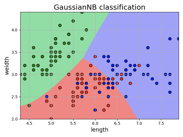
def plot_data(x, y, model):''':param x: 训练数据x:param y: 训练数据y:param mdoel: 模型:return:'''N, M = 500, 500 # 横纵各采样多少个值x1_min, x1_max = x[:, 0].min(), x[:, 0].max() # 第0列的范围x2_min, x2_max = x[:, 1].min(), x[:, 1].max() # 第1列的范围t1 = np.linspace(x1_min, x1_max, N)t2 = np.linspace(x2_min, x2_max, M)x1, x2 = np.meshgrid(t1, t2) # 生成网格采样点x_test = np.stack((x1.flat, x2.flat), axis=1) # 测试点mpl.rcParams['font.sans-serif'] = [u'simHei']mpl.rcParams['axes.unicode_minus'] = Falsecm_light = mpl.colors.ListedColormap(['#77E0A0', '#FF8080', '#A0A0FF'])cm_dark = mpl.colors.ListedColormap(['g', 'r', 'b'])y_hat = model.predict(x_test) # 预测值y_hat = y_hat.reshape(x1.shape) # 使之与输入的形状相同plt.figure(facecolor='w')plt.pcolormesh(x1, x2, y_hat, cmap=cm_light) # 预测值的显示plt.scatter(x[:, 0], x[:, 1], c=np.squeeze(y), edgecolors='k', s=50, cmap=cm_dark) # 样本的显示plt.xlabel('length', fontsize=14)plt.ylabel('weidth', fontsize=14)plt.xlim(x1_min, x1_max)plt.ylim(x2_min, x2_max)plt.title('GaussianNB classification', fontsize=18)plt.grid(True)plt.show()
主函数
if __name__ == '__main__':x, y = load_data('../data/iris.data')model = build_model()model.fit(x, y.ravel())plot_data(x, y, model)# 训练集上的预测结果y_hat = model.predict(x)y = y.reshape(-1)result = y_hat == yprint(y_hat)print(result)acc = np.mean(result)print('准确度: %.2f%%' % (100 * acc))
分类结果
准确度: 78.00%
代码位置

若有收获,就点个赞吧
0 人点赞
