Matrices 矩阵

1 如何看待线性方程

例如求解如下线性方程：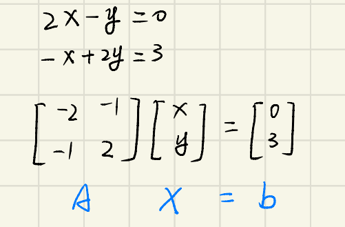

我们有两种看待方式，行图像（Row Picture）与列图像（Column Picture）。

1. Row Picture

就是中学学的，看作是两条直线的交点：

最终得到解就是交点坐标

1. Column Picture

这是重中之重，是理解线性代数后面部分的基石。看作两个列向量的线性组合（linear combination of columns）。转变成求解：

求出来 x=1, y=2

【求解线性方程问题】

Can I solve for every b?
==>
Do linear combinations of the columns of fill 3-D space?

2 矩阵乘法、初等矩阵与消元

2.1 Matrix multiplication 矩阵乘法

一共有四种计算矩阵乘法的方式。假设现在要求：

【第一种】 的一行乘以 一列

这是国内大学课本里面教的，也是最难用的！！

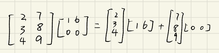
【第二种】 中的每一个列向量，都是 所有列向量的线性组合

将 和 写成列向量的形式：

进而有：
,

【第三种】 中的每一个行向量，都是 所有行向量的线性组合

,

【第四种】

第二种和第三种适合理解，而这一种最适合计算！

2.2 Elementary matrix & Elimination 初等矩阵与消元

考虑求解如下的线性方程

求解过程如下：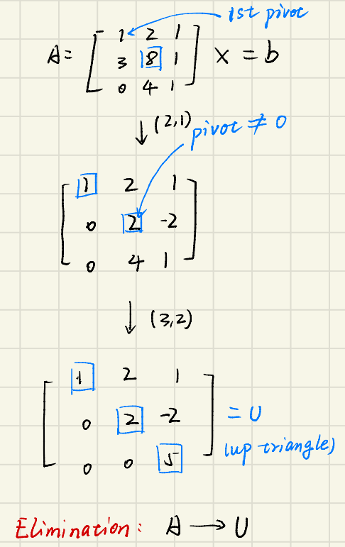

消元的结果是将矩阵 转换成了上三角矩阵（upper triangular matrix）。

上面的第一步对 矩阵的第二行进行操作 ，在图中使用 进行标识。其效果等效于使用一个初等矩阵 乘以矩阵 ：

这一点可以通过第三种矩阵乘法来解释：将矩阵 的三个行向量分别用 来表示，消元后的结果矩阵的第二个行向量 是 的线性组合，组合方式由初等矩阵 的第二行决定，即：

初等矩阵就是由单位阵（identity matrix）经过一次变换得到的矩阵，初等变换包括三种：

• 交换矩阵中某两行（列）的位置
• 用一个非零常数 k 乘以矩阵的某一行（列）
• 将矩阵的某一行（列）乘以常数k后加到另一行（列）上去

所以初等矩阵的逆矩阵也很好求，把对应的操作元变成相反数就可以。比如上面的 :

3 Inverse 逆矩阵

Invertible matrix 可逆矩阵（nonsingular matrix 非奇异矩阵）首先一定是方阵。

Invertible: we can solve only when 。也就是说 的列向量线性无关。

逆否命题 non-invertible: we can find that 。证明如下：

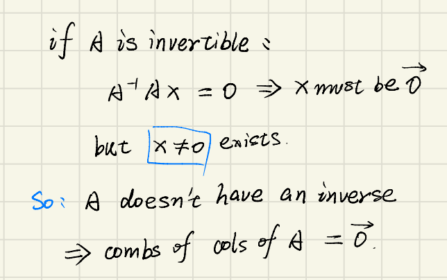
【逆矩阵的求法】Gauss-Jordan 法

Augmented matrix 增广矩阵。

方法正确性验证如下：

4 Factorization into A=LU LU分解

通过高斯消元法，我们将 中的矩阵 转换成了一个上三角阵（upper diagonal），比如：

可以转化成

因为初等变换阵的逆矩阵很好求，如果是乘数，则直接在相应位置求相反数就可以（可参考 2.2 节）。
假设这其中没有初等阵是用来交换两行的，则我们可以轻松的求出 矩阵，比如

而

我们发现 矩阵其实就是以前 和 中的乘数取了一个相反数。当然，这是在没有初等阵是用来交换两行的这个前提之下的。可以发现， 是一个下三角矩阵（lower diagonal）。

5 Solving Ax=b 解线性方程组 Ax=b

5.1 Solving Ax=0 解 Ax=0

假设 矩阵为：

用解方程的高斯消元法，逐步迭代，有：

最后一步我们总会得到一个上三角矩阵 ，被称为 echelon 阶梯矩阵，当然按照正常解方程的步骤应该还有一步是把矩阵 中的主元（pivot），尽可能都化成 1，但是这里为了简单表示就少了这一步。在上三角矩阵 中，有两列 有 pivot，而 这两列没有 pivot，所以 代表的列被称为 povit columns，相应 两个变量被称为 pivot variables，而 被称为 free variables.

在矩阵中有一个非常重要的概念叫秩 （Rank），，等于 pivot variable 的数量。上例中，。

回到解方程，在大学学的线性代数中，我们可以让 free variables 任意取值，然后随之确定 pivot variables，这
样就确定了方程的解。

在一个 的矩阵中， 代表：

1. 我们有 个 free variables
2. 在 这个方程中，只有 个独立的方程组（有用的）

所以解 的步骤：

1. 消元（elimination）
2. 找到 free variables （顺便可以找到 pivot variables）
3. 为 free variables 选择相互独立的组合（），并且解出对应的 pivot variables，一共有 个，记为
4. 最后使用任意变量 做一个线性组合就得到了最终的解：

   在上例中，，一共有 2 两个 free variables ，所以分别做两个独立的组合：令 以及 ，这样可以求解出两个特解 ，最后得出 的解为 ，其中 是任意实数。

上面 实际上长成了矩阵 的 nullspace，上面为 free variables 选取相互独立的组合，就是为了解出来的特解 是相互独立的，这样再进行线性组合得到 ，就长成了矩阵 的 nullspace。

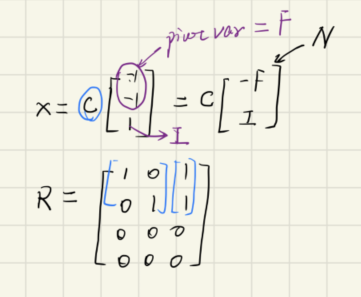
由所有特解组成的矩阵 就是作为矩阵 的 nullspace 矩阵，里面的向量就是 nullspace 的基底。而确定了空间的基地，就相当于确定了整个空间：

最后 的解可以写成这样：

其中 是 的矩阵， 是用来组合 个基底的 维向量，而且 是 任意的向量，因为 ，即 矩阵乘以任何一个特解 都等于零。

由此还可以看出，矩阵 A 的 nullspace 是 中的一个 维子空间。

Reduced row echelon form: pivot 位置的元素为 1，pivot 位置上下元素全都是 0，也就是我们从初中开始解方程组的形式

通过 矩阵可以快速求出 nullspace 矩阵 ：

5.2 Solving Ax=b 解 Ax=b

还是用上面的 矩阵：

上图最后一步得到的增广矩阵中，如果 ，则方程组有解，否则无解，因为 ，等式右边必须是 。

如果 有解（solvability），则需要满足以下任意一个条件（实际上是对 向量的条件）：

1. 在矩阵 的列空间 中
2. 如果在 的 reduced echelon form 矩阵 中某几行的元素全都是 ，那么算出来的增广矩阵中 向量一侧的那一个元素也必须是

的解 ，即特解 + 通解。

对于 ，当 取不同值时的解的情况（假设秩 ），首先进行讨论：
1. 列满秩（）：解为 1 个或 0 个，如果有解 ，解为特解且唯一

• nullspace 中只有零向量，没有 free variables
• 的列空间正好是 中的一个 维空间，所以如果向量 在 中则有解，否则无解
  1. 行满秩（）：一定有解，一个或无数个
• 长成了 ，所以向量 一定在 中
• 如果 ，则一定存在 free variables，此时有无数个解
  1. 矩阵 可逆：对于任何 有且仅有一个解

综上（ 代表 矩阵的 reduced row echelon）：

1. 当 时，，有且仅有一个解
2. 当 时，，有一个解或无解
3. 当 时，，有无数个解
4. 当 时，，无解或有无数个解

6 投影矩阵与最小二乘

6.1 Projection 投影与投影矩阵

为什么我们需要投影？—- 可能没有解，但我们可以将 投影到 的列空间 上，求解 来近似求解线性方程。

首先考虑投影到一维空间（一条直线）的情况，将向量 投影到 上。

最终 在 向量上的投影为 。所以我们定义在投影到一维空间的投影矩阵（projection matrix）

投影矩阵有如下性质：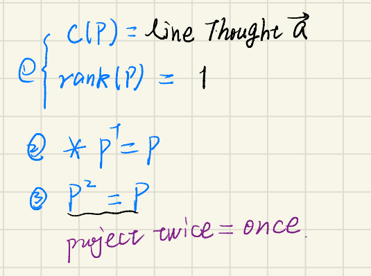

代表矩阵 的 column space.

随后考虑投影到二维空间（一个平面）的情况，将向量 投影到 形成的平面上。

得到 projection matrix 投影矩阵：

6.2 Least Square 最小二乘

最小二乘的思想：找到一条直线来拟合数据点，使得所有点到直线的距离平方和最小，比如：

最小化目标函数为：

当然，求解这个问题可以直接用求偏导等于零来计算：

得到：

还有就是投影的思想，的出来的 表达式跟上面的一样。最后求出来：

7 正交矩阵与 Gram-Schmidt 标准正交化

7.1 Orthogonal Matrix Q 正交矩阵

正交矩阵重要的性质：
%22%20aria-hidden%3D%22true%22%3E%0A%20%3Cuse%20xlink%3Ahref%3D%22%23E1-MJMATHI-51%22%20x%3D%220%22%20y%3D%220%22%3E%3C%2Fuse%3E%0A%20%3Cuse%20transform%3D%22scale(0.707)%22%20xlink%3Ahref%3D%22%23E1-MJMATHI-54%22%20x%3D%221119%22%20y%3D%22583%22%3E%3C%2Fuse%3E%0A%20%3Cuse%20xlink%3Ahref%3D%22%23E1-MJMATHI-51%22%20x%3D%221389%22%20y%3D%220%22%3E%3C%2Fuse%3E%0A%20%3Cuse%20xlink%3Ahref%3D%22%23E1-MJMAIN-3D%22%20x%3D%222458%22%20y%3D%220%22%3E%3C%2Fuse%3E%0A%20%3Cuse%20xlink%3Ahref%3D%22%23E1-MJMATHI-49%22%20x%3D%223515%22%20y%3D%220%22%3E%3C%2Fuse%3E%0A%3C%2Fg%3E%0A%3C%2Fsvg%3E#card=math&code=Q%5ET%20Q%20%3D%20I&id=qBj1Y)
同时，如果 是方阵，则

如果将 投影到正交矩阵的列空间 中，则：

得到的结果就是，向量 的每一个分量 ，其实就是点 在坐标轴 上的坐标：

7.2 Gram-Schmidt 标准正交化

先正交化，然后再标准化。

前者就是投影，后者就是向量除以模长

首先是两个向量标准正交化的步骤：

上图我们最终想要求的是与向量 垂直的分量

最后推广到三个向量：

8 行列式、性质与计算公式

8.1 Determinant & Properties 行列式及其性质

Determinant 行列式的表示：

行列式的 10 条性质：3 条定义 + 7 条定理（由定义推出来的）

8.2 Formula for detA 行列式计算公式

使用上述 10 条性质推到公式！！！

首先是二阶矩阵的行列式：

经过分解，我们将原始的行列式拆成了 4 个行列式的和。

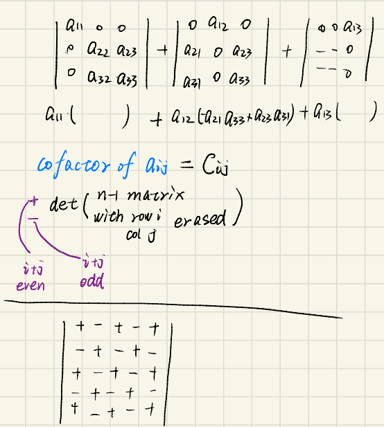
然后是三阶矩阵的行列式：

这里我们拆成了 33 个行列式的和

计算公式如下：

依次从每一行选择一个元素，各个元素的列不重复。

一旦上面选择的某一个元素为 0，那它代表的行列式就等于 0（因为有一列全零）。

8.3 Cofactors 代数余子式

使用伴随矩阵求逆矩阵：

9 Eigen value & vector 特征值与特征向量

1. 使用矩阵乘以该矩阵的 eigen vector，其结果与原来的向量平行，只是进行了缩放操作
2. #pivots = #independent cols = **#λ's = #different eigen vectors**
   1. 所以如果找到一组 eigen vector 组成的基底，将其他向量用该基底进行表示，就能使用上面矩阵幂次来大大简化计算

特征值与特征向量的计算：

矩阵的 trace 迹、特征值的积：

10 对角化与矩阵 A 的幂

10.1 DIagonalization 对角化

既然有特征值，那 **A** 一定是一个方阵。

其中 为 的 n 个独立的特征向量组成的矩阵。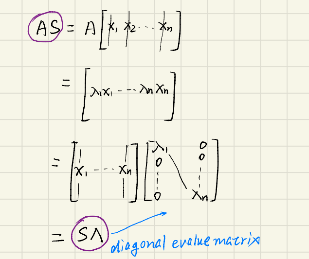

最终推出：

只要保证 的 **n** 个特征值不同，即可保证有 **n** 个独立的特征向量。

10.2 Power of A 矩阵 A 的幂

从 很容易得到 ：

进而对于给定 以及等式 ，我们有

如果想求 的值，首先将 的特征向量 看作一组基底，然后用这组基底表示 ：

那么

这个式子很有用：如果 ，则它代表的这一项 。

比如计算斐波那契数列增长的速度：

11 Markov matrix

1. 所有的元素
2. 每一列元素和都是

性质：

1. 是一个特征值，其余所有的 均

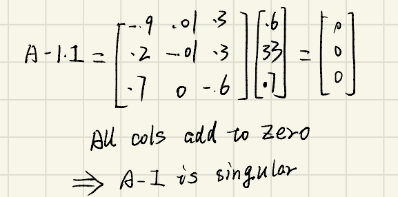
1. 所以根据 9.2 节 Power of A， 最终会达到一个稳定状态。

实例：

12 SVD 奇异值分解

Singular Value Decomposition.

其中 都是正交矩阵。

思想：设 ，

分别是矩阵 的 row space 和 column space 的正交基向量组成的基底。希望通过 完成：

即

如何求解三个矩阵？

首先求 ：

然后求 :

13 Linear transformation & their matrices 线性变换

线性性：

向量的各个分量、一个点坐标的意义；只有确定了基底，坐标才有意义：

进一步，

其中 的各列，其实就是 轴的单位向量。

线性变换，相当于变化坐标轴（也就是基底），而点的坐标保持不变。比如二维空间中逆时针旋转 的旋转矩阵：

看下图：

可以看到， 在新坐标系 中的坐标还是 。假设变换后的 轴和 轴的单位向量为 ，那么在新的坐标系下依旧有：

而新的 轴和 轴的单位向量，在原 坐标系下的坐标为：

OK，点到为止。

线性变换，线性说的是一件什么事：假如我们用函数 代表线性变换，则线性变换有如下性质：

所以有：

即对 和 的线性组合进行线性变换，其结果等于先进行线性变换，再进行线性组合。

结合上面旋转矩阵的例子，有点意思。这里 就可以理解为两个基向量，组成一组基底；而 则是向量在原基底 和新基底 中的坐标，没有发生变化！！