paper：Unleashing the Power of Contrastive Self-Supervised Visual Models via Contrast-Regularized Fine-Tuning
database：https://github.com/Vanint/Core-tuning

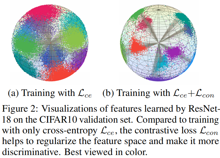
这篇是NIPS21的论文，来自新国立和中科大。

简介

融合Contrastive loss和CE loss

本文是对于传统的CE loss进行了改进，作者认为传统的CE loss在进行微调的时候，会最大类间距离，对于减少类内距离则能力不足。

cross-entropy tends to separate inter-class features, the resulting models still have limited capability for reducing intra-class feature scattering that exists in CSL models.

对于这种问题，作者提出在微调的时候融合对比学习的loss(式1)和ce loss

总的就是。

正负样本生成策略

此外，作者认为微调的下游任务有时候过于简单，可能导致Contrastive loss学不到好的东西，作者提出了一个难样本生成的策略（Core-tuning），这样可以增加Contrastive loss的作用。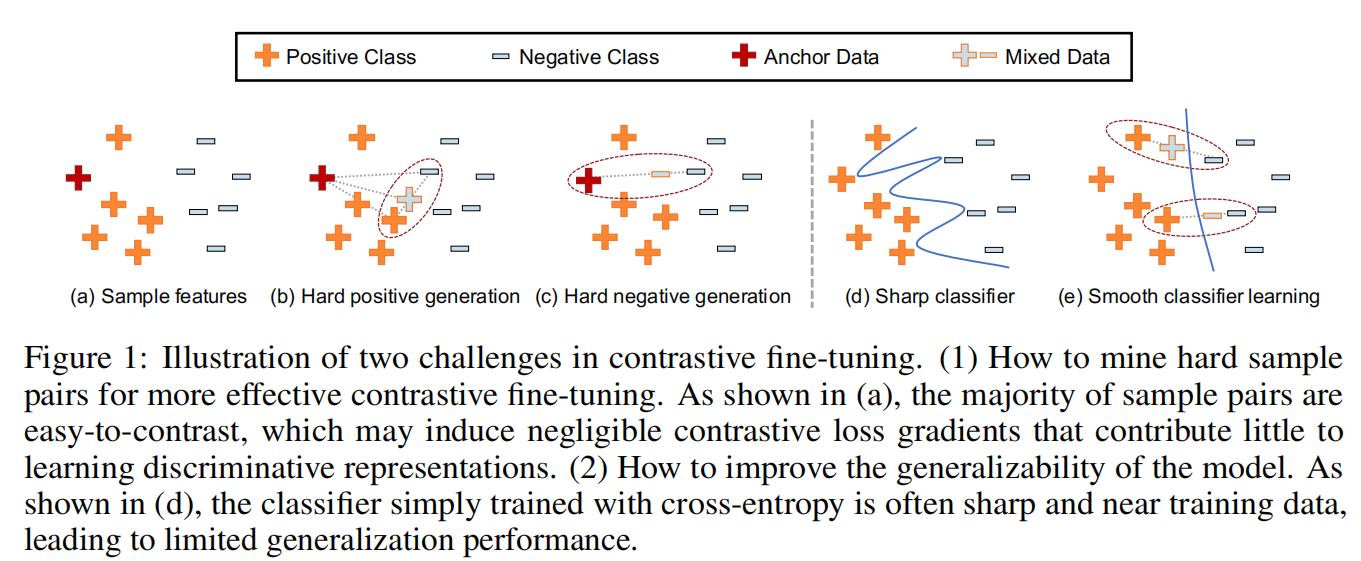

决策面的光滑

因为有文献表明ce loss学出来的决策面会很陡峭（sharp）。作者使用类似mixup的方法，对样本进行改造，并更改ce loss的形式（加入了生成的难样本的部分）。

Instead of simply adding the contrastive loss to the objective of fifine-tuning, Core-tuning further applies a novel hard pair mining strategy for more effective contrastive fifine-tuning, as well as smoothing the decision boundary to better exploit the learned discriminative feature space.

Contrastive Loss

作者使用的是有监督的Contrastive loss，是一种InfoNCE的变体：

这里的分别表示正样本对和所有的样本对（包含正负样本对），是锚特征（anchor feature）。相同类的feature（）为正样本对，不同类的为负样本对。是温度系数。

Contrastive loss的正则化作用

作者给出了下面的定理，认为Contrastive loss有正则化作用：

是norm之后的特征，标签。
最小化，可以减小类内的熵，使得每一类的feature分布地更加紧密。
最大化，可以增大内间的熵，使得不同类的feature分布地更加分散。

Contrastive loss的优化作用

作者给出了定理2，认为正比于条件交叉熵减：
:::info 条件交叉熵为。交叉熵为： ::: 是模型预测的标签。
因为是数据给定了的，所以第二项可以忽略。因此最小化等价于最小化条件交叉熵。直觉上可以认为，这样可以将正样本拉近，负样本推开，使得预测的标签的分布更加满足真实标签的分布。

More intuitively, pulling positive pairs together and pushing negative pairs further apart make the predicted label distribution closer to the ground-truth distribution, which further minimizes the cross-entropy loss.

对比正则微调（Contrast-Regularized Tuning）

作者发现对于小于任务微调的时候，由于有时候任务较为简单，导致Contrastive loss梯度几乎为0，导致其没有起到作用，作者这里提出了生成难样本的方法。具体而言，生成难正样本和难负样本。

难正样本的生成

对于每一个给定的anchor feature，基于余弦距离找到最难的正样本（最大距离）最难（最小距离）的负样本。根据式3生成难正样本：

难负样本的生成

对于每一个给定的anchor feature，随机采样一个负样本作为最难的负样本。生成的难负样本（semi-hard negatives）如下：


作者这里说明，随机挑选而不是挑选最难的负样本是因为使用最难的负样本会导致性能的降低。

难样本对的权重调整

在生成难样本对之后，作者使用额外的两层MLP得到对比的feature（contrastive feature）。

这里可能是遵循了对比学习的做法，增加一个projection head。

并且对于难正样本增加了权重，但由于难样本对会降低预测精度，作者follow了一下focal loss的做法，添加了一项权重。最终改写为式5：

样本越难，越小（在0到1之间），越大，越小（为负），不加权重的越大，乘上之后，能将相对减小。

分类器决策面的光滑化（smooth）

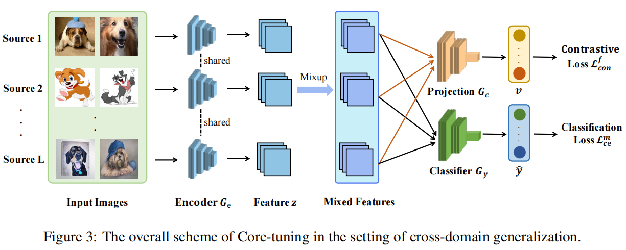
作者受到mixup的启发，使用混合之后的数据（原始样本和生成的难样本）训练网络。并将ce loss改为下面的形式：

就是加的额外的2层的MLP（projection head）。

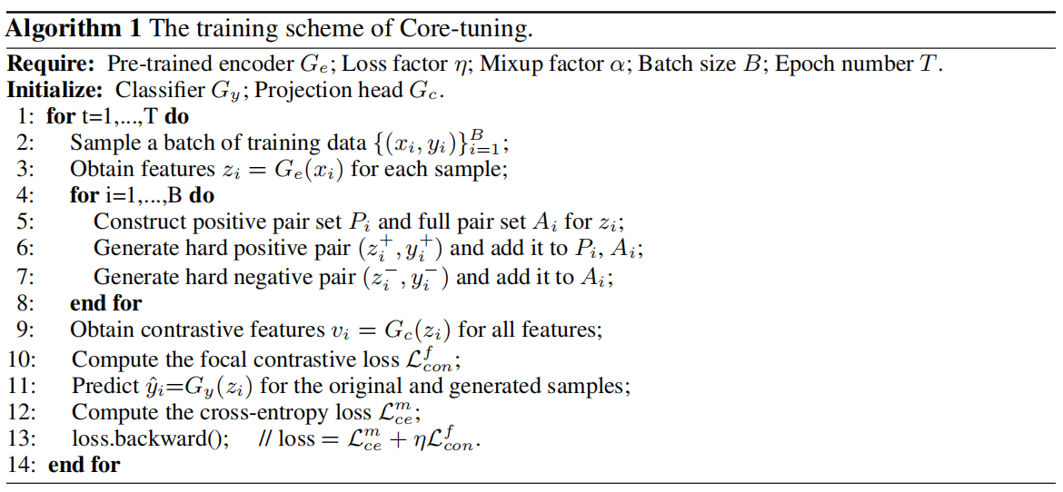
伪代码

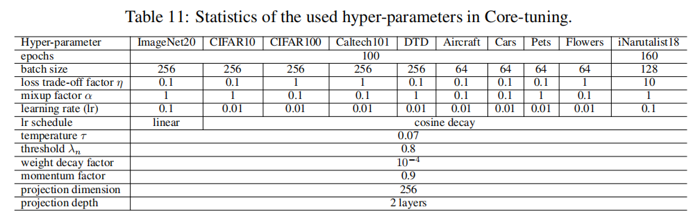
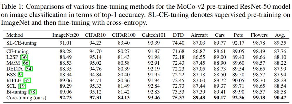
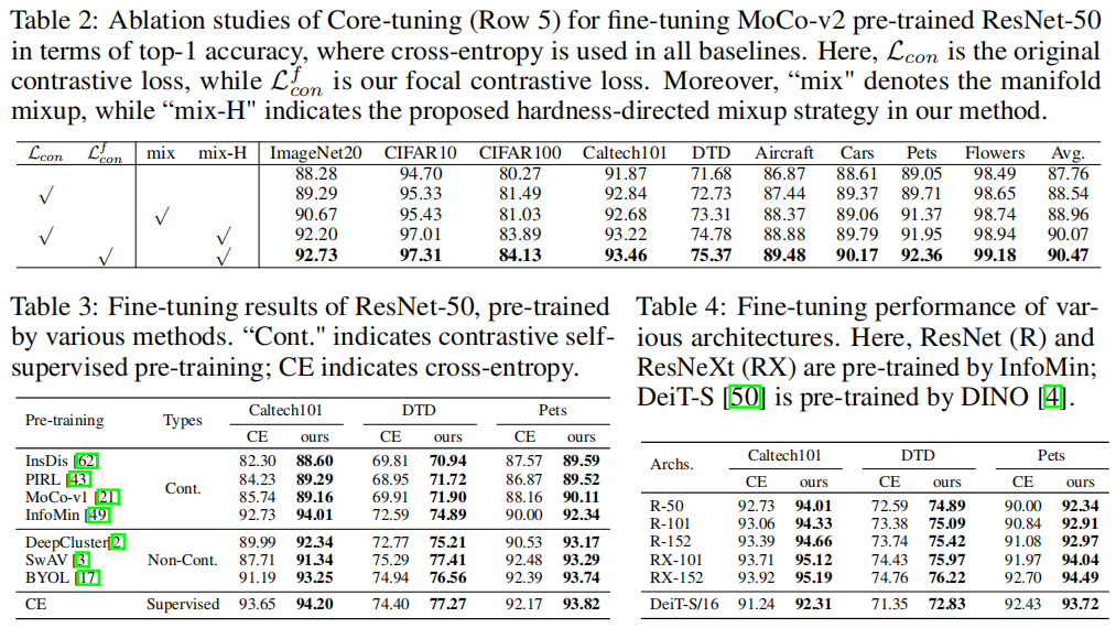
实现细节及表现

定理推导

这篇文章的推导看起来很奇怪，可能是我水平有限。

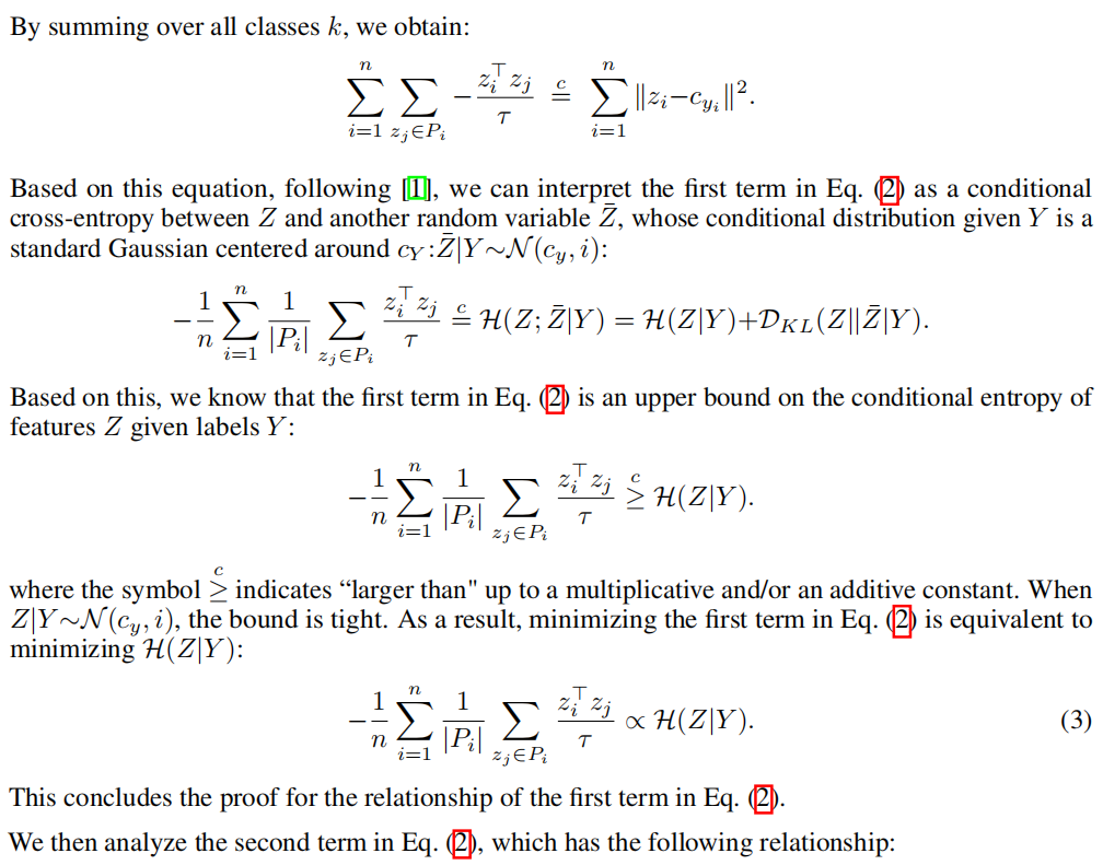
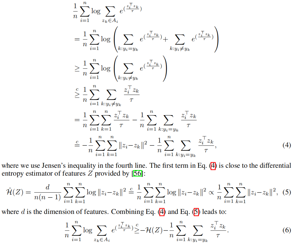
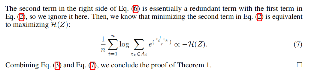
定理1

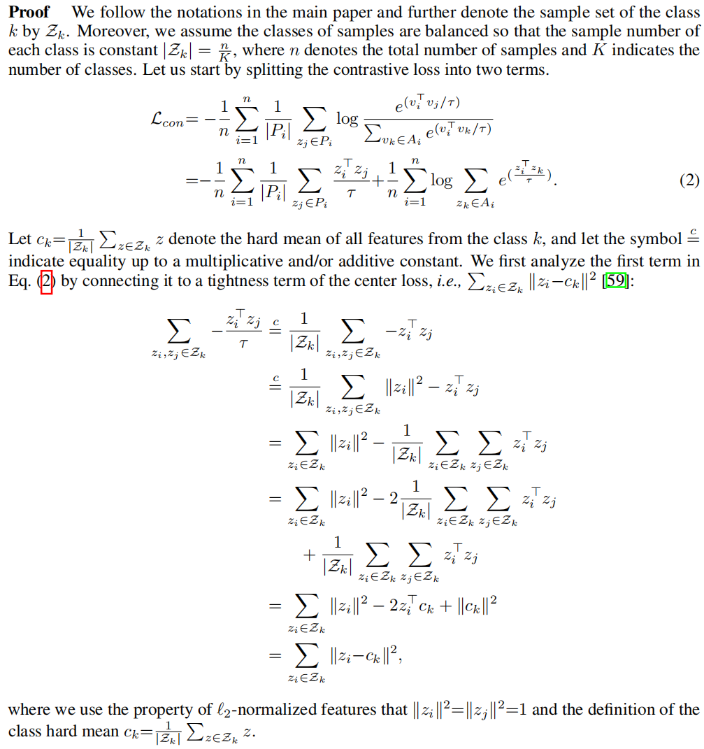
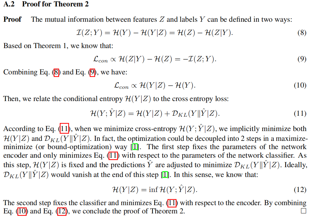
定理2