1 导入数据,探索数据
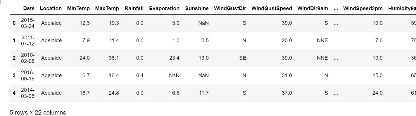
import pandas as pdimport numpy as npfrom sklearn.model_selection import train_test_splitweather = pd.read_csv(r"C:\Users\18700\Desktop\08支持向量机下\weatherAUS5000.csv",index_col=0)weather.head() #默认查看前5行
#将特征矩阵和标签Y分开X = weather.iloc[:,:-1]Y = weather.iloc[:,-1]X.shape#探索数据类型 查看缺失X.info()#探索缺失值X.isnull().mean() #.mean()可以直接查看缺失值占总值的比例 isnull().sum(全部的True)/X.shape[0]#可以看到需要不同的填补策略
输出结果
Date 0.0000Location 0.0000MinTemp 0.0042MaxTemp 0.0026Rainfall 0.0100Evaporation 0.4318Sunshine 0.4858WindGustDir 0.0662WindGustSpeed 0.0662WindDir9am 0.0698WindDir3pm 0.0226WindSpeed9am 0.0102WindSpeed3pm 0.0162Humidity9am 0.0128Humidity3pm 0.0240Pressure9am 0.0988Pressure3pm 0.0992Cloud9am 0.3778Cloud3pm 0.3976Temp9am 0.0066Temp3pm 0.0176dtype: float64
Y.isnull().sum() #返回要不是0,就是有空值#探索标签的分类np.unique(Y) #可以看到标签是二分类
2 分集,优先探索标签
分训练集和测试集,并做描述性统计
#分训练集和测试集Xtrain, Xtest, Ytrain, Ytest = train_test_split(X,Y,test_size=0.3,random_state=420)#恢复索引for i in [Xtrain, Xtest, Ytrain, Ytest]:i.index = range(i.shape[0])
先看标签是否存在问题
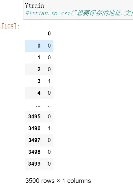
#是否有样本不平衡问题?Ytrain.value_counts() #查看Ytest.value_counts()#可以看到有轻微的样本不均衡问题#将标签编码from sklearn.preprocessing import LabelEncoder #标签专用,第三章讲过encorder = LabelEncoder().fit(Ytrain) #LabelEncoder允许一维数据输入#构成的模型认得了:有两类:YES和NO,YES是1,NO是0,因为YES是少数类#使用训练集进行训练,然后在训练集和测试集上分别进行transform:相当是用训练集的训练结果分别对测试集和训练集进行改造Ytrain = pd.DataFrame(encorder.transform(Ytrain)) #将Ytrain转换维0,1,然后放回到Ytrain中Ytest = pd.DataFrame(encorder.transform(Ytest))#如果测试集中出现了训练集中没有出现过的标签类型,比如unkown,这时LabelEncoder就会报错。#如果报错就要重新分训练集和测试集Ytrain#Ytrian.to_csv("想要保存的地址.文件名.csv") #一般先将标签保存了,再去做其它的操作

3 探索特征,开始处理特征矩阵
3.1 描述性统计和异常值
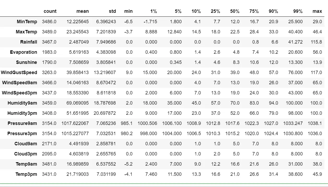
#描述性统计 通过观察最小值和1%,最大值和99%值之间的差异,可以判断出是否有数据偏差和异常值Xtrain.describe([0.01,0.05,0.1,0.25,0.5,0.75,0.9,0.99]).TXtest.describe([0.01,0.05,0.1,0.25,0.5,0.75,0.9,0.99]).T
3.2 处理异常值思路
#处理异常值思路:如果有异常值,需要先看异常值出现的频率,如果只有一次,多半时输入错误,这种情况,直接删除;#如果出现多次,需要和业务人员沟通。人为造成的异常值时没有用的,需要删除。#有时异常值很多10%以上,我需要将异常值替换成非干扰项:比如用0或者把异常值当缺失值,用均值或者众数来填补。#先查看原始的数据结构Xtrain.shapeXtest.shape#观察异常值是大量存在,还是少数存在Xtrain.loc[Xtrain.loc[:,"Cloud9am"] == 9,"Cloud9am"]Xtest.loc[Xtest.loc[:,"Cloud9am"] == 9,"Cloud9am"]Xtest.loc[Xtest.loc[:,"Cloud3pm"] == 9,"Cloud3pm"]#少数存在,于是采取删除的策略#注意如果删除特征矩阵,则必须连对应的标签一起删除,特征矩阵的行和标签的行必须要一一对应Xtrain = Xtrain.drop(index = 71737)Ytrain = Ytrain.drop(index = 71737)#删除完毕之后,观察原始的数据结构,确认删除正确Xtrain.shapeXtest = Xtest.drop(index = [19646,29632])Ytest = Ytest.drop(index = [19646,29632])Xtest.shape#进行任何行删除之后,千万记得要恢复索引for i in [Xtrain, Xtest, Ytrain, Ytest]:i.index = range(i.shape[0])Xtrain.head()Xtest.head()
3.3 首先处理困难特征:日期
#处理困难特征日期type(Xtrain.iloc[0,0]) #字符串#首先需要探索日期时连续性还是分类型特征#日期是一年分了365类的分类型变量#判断日期中是否有重复,Xtrain.iloc[:,0].value_counts() #日期不是连续型,是有重复的
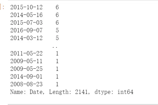
Xtrain.iloc[:,0].value_counts().count()#2141##如果我们把它当作分类型变量处理,类别太多,有2141类,如果换成数值型,会被直接当成连续型变量,如果做成哑变量,我们特征的维度会爆炸#所以日期不能单纯的当作连续型或者分类型,所以如果认为没有用的话,可以删除#Xtrain = Xtrain.drop(["Date"],axis=1)#Xtest = Xtest.drop(["Date"],axis=1)
3.3.1 将样本对应标签之间的联系,转换成是特征与标签之间的联系
Xtrain["Rainfall"].head(20)#通过描述性表格可以看下,可以设置大于1mm就是下雨了Xtrain["Rainfall"].isnull().sum() #可以看到有空值Xtrain.loc[Xtrain["Rainfall"] >= 1,"RainToday"] = "Yes" #因为没有这一列RainToday,会自己添加Xtrain.loc[Xtrain["Rainfall"] < 1,"RainToday"] = "No"Xtrain.loc[Xtrain["Rainfall"] == np.nan,"RainToday"] = np.nan #将空值就赋值空值Xtest.loc[Xtest["Rainfall"] >= 1,"RainToday"] = "Yes"Xtest.loc[Xtest["Rainfall"] < 1,"RainToday"] = "No"Xtest.loc[Xtest["Rainfall"] == np.nan,"RainToday"] = np.nanXtrain.head()
Xtrain.loc[:,"RainToday"].value_counts()Xtest.head()Xtest.loc[:,"RainToday"].value_counts()
输出结果
No 2642Yes 825Name: RainToday, dtype: int64
3.3.2 创造第二个特征month
int(Xtrain.loc[0,"Date"].split("-")[1]) #提取出一个月份 int就是将提取的月份字符元素变为整数Xtrain["Date"] = Xtrain["Date"].apply(lambda x:int(x.split("-")[1]))#apply是对dataframe上某一列进行处理的一个函数#lambda 是匿名函数,lambda x是请在dataframe上这一列中的每一行执行冒号后面的命令Xtrain.loc[:,"Date"].value_counts() #可以看到变成了12个数字的分类型变量
输出结果
3 3345 3247 3169 3026 3021 30011 29910 2824 2652 26412 2598 253Name: Date, dtype: int64
#替换完毕后,我们需要修改列的名称#rename是比较少有的,可以用来修改单个列名的函数#我们通常都直接使用 df.columns = 某个列表 这样的形式来一次修改所有的列名#但rename允许我们只修改某个单独的列Xtrain = Xtrain.rename(columns={"Date":"Month"}) #里面是一个字典Xtrain.head()
#所有的操作要在测试集也运行下Xtest["Date"] = Xtest["Date"].apply(lambda x:int(x.split("-")[1]))Xtest = Xtest.rename(columns={"Date":"Month"})Xtest.head()
3.4 处理困难特征:地点
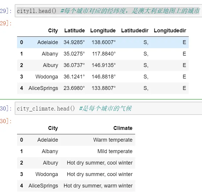
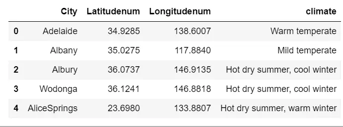
Xtrain.loc[:,"Location"].value_counts().count() #超过25个类别的变量,都会被算法当成连续性变量,所以现在用地点分是不行的#49#我们有了澳大利亚全国主要城市的气候,也有了澳大利亚主要城市的经纬度(地点),我们就可以通过计算我们样#本中的每个气候站到各个主要城市的地理距离,来找出一个离这个气象站最近的主要城市,而这个主要城市的气候#就是我们样本点所在的地点的气候。#让我们把cityll.csv和cityclimate.csv来导入,来看看它们是什么样子:cityll = pd.read_csv(r"C:\Users\18700\Desktop\08支持向量机下\cityll.csv",index_col=0)city_climate = pd.read_csv(r"C:\Users\18700\Desktop\08支持向量机下\Cityclimate.csv")cityll.head() #每个城市对应的经纬度,是澳大利亚地图上的城市city_climate.head() #是每个城市的气候
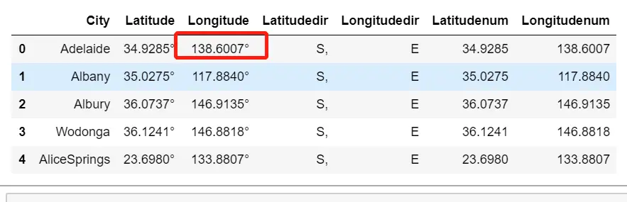
#去掉度数符号cityll["Latitudenum"] = cityll["Latitude"].apply(lambda x:float(x[:-1])) #x[:-1]对纬度进行切片cityll["Longitudenum"] = cityll["Longitude"].apply(lambda x:float(x[:-1]))cityll.head()
#观察一下所有的经纬度方向都是一致的,全部是南纬,东经,因为澳大利亚在南半球,东半球,所以经纬度的方向我们可以舍弃了citylld = cityll.iloc[:,[0,5,6]] #取出城市名称和经纬度#将city_climate中的气候添加到我们的citylld中citylld["climate"] = city_climate.iloc[:,-1]citylld.head()
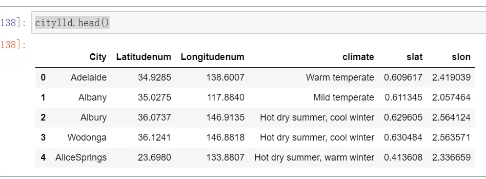
#看下爬虫下来的训练集中所有地点的表格:samplecity = pd.read_csv(r"C:\Users\18700\Desktop\08支持向量机下\samplecity.csv",index_col=0)samplecity.head()#我们对samplecity也执行同样的处理:去掉经纬度中度数的符号,并且舍弃我们的经纬度的方向samplecity["Latitudenum"] = samplecity["Latitude"].apply(lambda x:float(x[:-1]))samplecity["Longitudenum"] = samplecity["Longitude"].apply(lambda x:float(x[:-1]))samplecityd = samplecity.iloc[:,[0,5,6]]samplecityd.head()#我们现在有了澳大利亚主要城市的经纬度和对应的气候,也有了我们的样本的地点所对应的经纬度,接下来#我们要开始计算我们样本上的地点到每个澳大利亚主要城市的距离#首先使用radians将角度转换成弧度from math import radians, sin, cos, acoscitylld.loc[:,"slat"] = citylld.iloc[:,1].apply(lambda x : radians(x)) #将维度准换维为弧度citylld.loc[:,"slon"] = citylld.iloc[:,2].apply(lambda x : radians(x))samplecityd.loc[:,"elat"] = samplecityd.iloc[:,1].apply(lambda x : radians(x))samplecityd.loc[:,"elon"] = samplecityd.iloc[:,2].apply(lambda x : radians(x))samplecityd.head()citylld.head()
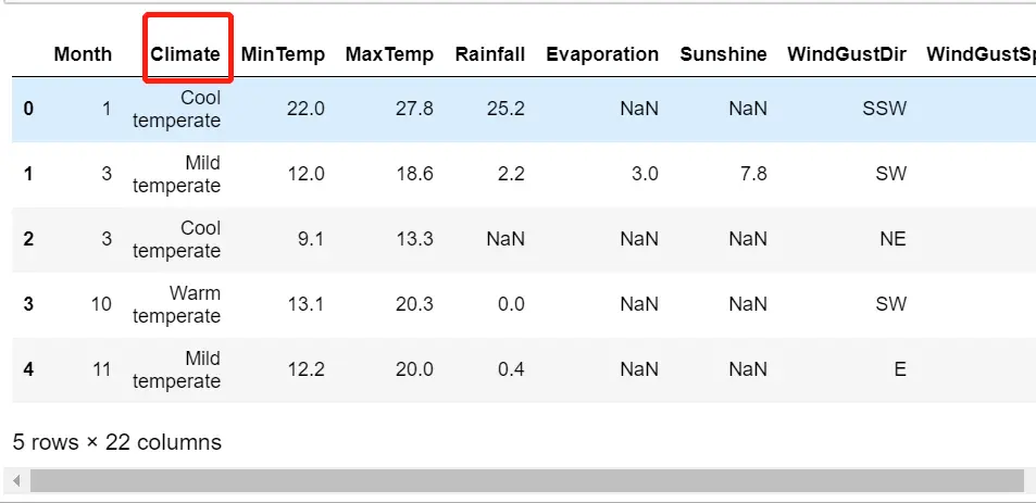
#查看气候的分布samplecityd["climate"].value_counts()#确认无误后,取出样本城市所对应的气候,并保存locafinal = samplecityd.iloc[:,[0,-1]]locafinal.columns = ["Location","Climate"]locafinal.head()#在这里设定locafinal的索引为地点,是为了之后进行map的匹配locafinal = locafinal.set_index(keys="Location")locafinal.head()#locafinal.to_csv(r"C:\work\learnbetter\micro-class\week 8 SVM (2)\samplelocation.csv") #然后将其保存#将location中的内容替换,并且确保匹配进入的气候字符串中不含有逗号,气候两边不含有空格#我们使用re这个模块来消除逗号#re.sub(希望替换的值,希望被替换成的值,要操作的字符串)#x.strip()是去掉空格的函数,将两边的空值都去掉import reXtrain["Location"] = Xtrain["Location"].map(locafinal.iloc[:,0]).apply(lambda x:re.sub(",","",x.strip()))Xtest["Location"] = Xtest["Location"].map(locafinal.iloc[:,0]).apply(lambda x:re.sub(",","",x.strip()))#修改特征内容之后,我们使用新列名“Climate”来替换之前的列名“Location”#注意这个命令一旦执行之后,就再没有列"Location"了,使用索引时要特别注意Xtrain = Xtrain.rename(columns={"Location":"Climate"})Xtest = Xtest.rename(columns={"Location":"Climate"})Xtrain.head()Xtest.head()#这时地点就变成了气候,并且只有7个气候的分类文字型特征
4 处理分类型变量:缺失值
在实际过程中,测试集和训练集的数据分布和性质都是相似的,因此我们统一使用训练集的众数和均值来对测试集进行填补。
#查看缺失值的缺失情况Xtrain.isnull().mean()Month 0.000000Climate 0.000000MinTemp 0.004000MaxTemp 0.003143Rainfall 0.009429Evaporation 0.433429Sunshine 0.488571WindGustDir 0.067714WindGustSpeed 0.067714WindDir9am 0.067429WindDir3pm 0.024286WindSpeed9am 0.009714WindSpeed3pm 0.018000Humidity9am 0.011714Humidity3pm 0.026286Pressure9am 0.098857Pressure3pm 0.098857Cloud9am 0.379714Cloud3pm 0.401429Temp9am 0.005429Temp3pm 0.019714RainToday 0.009429dtype: float64
首先找出分类特征
#首先找出,分类型特征都有哪些cate = Xtrain.columns[Xtrain.dtypes == "object"].tolist()cate#除了特征类型为"object"的特征们,还有虽然用数字表示,但是本质为分类型特征的云层遮蔽程度cloud = ["Cloud9am","Cloud3pm"]cate = cate + cloudcate#输出结果['Climate','WindGustDir','WindDir9am','WindDir3pm','RainToday','Cloud9am','Cloud3pm']
对于分类数据,使用众数来进行填补
#对于分类型特征,我们使用众数来进行填补from sklearn.impute import SimpleImputersi = SimpleImputer(missing_values=np.nan,strategy="most_frequent") #实例化#注意,我们使用训练集数据来训练我们的填补器,本质是在生成训练集中的众数si.fit(Xtrain.loc[:,cate]) #在分类数据上进行训练#然后我们用训练集中的众数来同时填补训练集和测试集Xtrain.loc[:,cate] = si.transform(Xtrain.loc[:,cate])Xtest.loc[:,cate] = si.transform(Xtest.loc[:,cate])Xtrain.head()Xtest.head()
#查看分类型特征是否依然存在缺失值Xtrain.loc[:,cate].isnull().mean() #可以看到已经没有缺失值了#输出结果Climate 0.0WindGustDir 0.0WindDir9am 0.0WindDir3pm 0.0RainToday 0.0Cloud9am 0.0Cloud3pm 0.0dtype: float64
处理分类型变量,将分类型变量编码
#将所有的分类型变量编码为数字,一个类别是一个数字from sklearn.preprocessing import OrdinalEncoder #只允许二维以上的数据输入的编码的类,区别于labelenconderoe = OrdinalEncoder()#利用训练集进行fitoe = oe.fit(Xtrain.loc[:,cate])#用训练集的编码结果来编码训练和测试特征矩阵#在这里如果测试特征矩阵报错,就说明测试集中出现了训练集中从未见过的类别Xtrain.loc[:,cate] = oe.transform(Xtrain.loc[:,cate])Xtest.loc[:,cate] = oe.transform(Xtest.loc[:,cate])Xtrain.loc[:,cate].head()Xtest.loc[:,cate].head()

5 处理连续性变量
1 填补缺失值
col = Xtrain.columns.tolist()#取出所有列的名称colfor i in cate:col.remove(i) #提出分类型列的名称col#实例化模型,填补策略为"mean"表示均值impmean = SimpleImputer(missing_values=np.nan,strategy = "mean")#用训练集来fit模型impmean = impmean.fit(Xtrain.loc[:,col])#分别在训练集和测试集上进行均值填补Xtrain.loc[:,col] = impmean.transform(Xtrain.loc[:,col])Xtest.loc[:,col] = impmean.transform(Xtest.loc[:,col])Xtrain.head()Xtest.head()Xtrain.isnull().mean() #可以看到已经没有缺失值了Xtest.isnull().mean() #可以看到已经没有缺失值了
输出结果
Month 0.0Climate 0.0MinTemp 0.0MaxTemp 0.0Rainfall 0.0Evaporation 0.0Sunshine 0.0WindGustDir 0.0WindGustSpeed 0.0WindDir9am 0.0WindDir3pm 0.0WindSpeed9am 0.0WindSpeed3pm 0.0Humidity9am 0.0Humidity3pm 0.0Pressure9am 0.0Pressure3pm 0.0Cloud9am 0.0Cloud3pm 0.0Temp9am 0.0Temp3pm 0.0RainToday 0.0dtype: float64
2 处理连续性变量:无量纲化
数据的无量纲化是SVM执行前的重要步骤,因此我们需要对数据进行无量纲化。但注意,这个操作我们不对分类型变量进行。
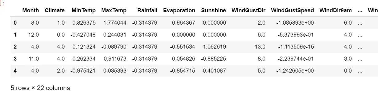
col.remove("Month") #因为不想把month也归一化colfrom sklearn.preprocessing import StandardScaler #把数据转换为均值为0,方差为1的数据;#标准化不改变数据的分布,不会把数据变成正态分布ss = StandardScaler()ss = ss.fit(Xtrain.loc[:,col])Xtrain.loc[:,col] = ss.transform(Xtrain.loc[:,col])Xtest.loc[:,col] = ss.transform(Xtest.loc[:,col])Xtrain.head()Xtest.head()
6 建模和模型评估
from time import time #随时监控运行时间import datetimefrom sklearn.svm import SVCfrom sklearn.model_selection import cross_val_scorefrom sklearn.metrics import roc_auc_score, recall_scoreYtrain = Ytrain.iloc[:,0].ravel() #需要将二维变为一维结构,如果是通过实现保存的csv导入的话Ytest = Ytest.iloc[:,0].ravel()#建模选择自然是我们的支持向量机SVC,首先用核函数的学习曲线来选择核函数#我们希望同时观察,精确性,recall以及AUC分数times = time() #因为SVM是计算量很大的模型,所以我们需要时刻监控我们的模型运行时间for kernel in ["linear","poly","rbf","sigmoid"]:clf = SVC(kernel = kernel,gamma="auto",degree = 1,cache_size = 5000).fit(Xtrain, Ytrain)result = clf.predict(Xtest) #首先获取模型结果score = clf.score(Xtest,Ytest) #接口socre返回accuracyrecall = recall_score(Ytest, result) #得到召回得分 输入(真实值,预测值)auc = roc_auc_score(Ytest,clf.decision_function(Xtest)) #得到auc(真实值,置信度)print("%s 's testing accuracy %f, recall is %f', auc is %f" % (kernel,score,recall,auc))print(datetime.datetime.fromtimestamp(time()-times).strftime("%M:%S:%f"))
7 模型调参
1 要求最高recall
#首先可以打开我们的class_weight参数,使用balanced模式来调节我们的recall:times = time()for kernel in ["linear","poly","rbf","sigmoid"]:clf = SVC(kernel = kernel,gamma="auto",degree = 1,cache_size = 5000,class_weight = "balanced").fit(Xtrain, Ytrain)result = clf.predict(Xtest)score = clf.score(Xtest,Ytest)recall = recall_score(Ytest, result)auc = roc_auc_score(Ytest,clf.decision_function(Xtest))print("%s 's testing accuracy %f, recall is %f', auc is %f" % (kernel,score,recall,auc))print(datetime.datetime.fromtimestamp(time()-times).strftime("%M:%S:%f"))#可以看到recall明显提升了,并且线性核最好
输出结果
linear 's testing accuracy 0.796667, recall is 0.775510', auc is 0.87006200:18:704683poly 's testing accuracy 0.793333, recall is 0.763848', auc is 0.87144800:21:757529rbf 's testing accuracy 0.803333, recall is 0.600583', auc is 0.81971300:30:587768sigmoid 's testing accuracy 0.562000, recall is 0.282799', auc is 0.43711900:35:731341
# 在锁定了线性核函数之后,我甚至可以将class_weight调节得更加倾向于少数类times = time()clf = SVC(kernel = "linear",gamma="auto",cache_size = 5000,class_weight = {1:10} #注意,这里写的其实是,类别1比例是10,隐藏了类别0:1,类别0比例是1).fit(Xtrain, Ytrain)result = clf.predict(Xtest)score = clf.score(Xtest,Ytest)recall = recall_score(Ytest, result)auc = roc_auc_score(Ytest,clf.decision_function(Xtest))print("testing accuracy %f, recall is %f', auc is %f" % (score,recall,auc))print(datetime.datetime.fromtimestamp(time()-times).strftime("%M:%S:%f"))#此时我们的目的就是追求一个比较高的AUC分数和比较好的recall,那我们的模型此时就算是很不错了
输出结果
testing accuracy 0.636667, recall is 0.912536', auc is 0.86636000:33:176004
2 追求平衡
#我们前面经历了多种尝试,选定了线性核,并发现调节class_weight并不能够使我们模型有较大的改善。现在我们#来试试看调节线性核函数的C值能否有效果:#需要运行很久import matplotlib.pyplot as pltC_range = np.linspace(0.01,20,10)recallall = []aucall = []scoreall = []for C in C_range:times = time()clf = SVC(kernel = "linear",C=C,cache_size = 5000,class_weight = "balanced").fit(Xtrain, Ytrain)result = clf.predict(Xtest)score = clf.score(Xtest,Ytest)recall = recall_score(Ytest, result)auc = roc_auc_score(Ytest,clf.decision_function(Xtest))recallall.append(recall)aucall.append(auc)scoreall.append(score)print("under C %f, testing accuracy is %f,recall is %f', auc is %f" % (C,score,recall,auc))print(datetime.datetime.fromtimestamp(time()-times).strftime("%M:%S:%f"))print(max(aucall),C_range[aucall.index(max(aucall))])plt.figure()plt.plot(C_range,recallall,c="red",label="recall")plt.plot(C_range,aucall,c="black",label="auc")plt.plot(C_range,scoreall,c="orange",label="accuracy")plt.legend()plt.show()
输出结果
under C 0.010000, testing accuracy is 0.800000,recall is 0.752187', auc is 0.87063400:02:383540under C 1.062105, testing accuracy is 0.796000,recall is 0.775510', auc is 0.87000900:18:778634under C 2.114211, testing accuracy is 0.794000,recall is 0.772595', auc is 0.87017800:32:681368under C 3.166316, testing accuracy is 0.795333,recall is 0.772595', auc is 0.87015800:45:965365under C 4.218421, testing accuracy is 0.795333,recall is 0.772595', auc is 0.87015301:00:687411under C 5.270526, testing accuracy is 0.795333,recall is 0.772595', auc is 0.87012801:13:145664under C 6.322632, testing accuracy is 0.796000,recall is 0.775510', auc is 0.87006001:15:696609under C 7.374737, testing accuracy is 0.795333,recall is 0.772595', auc is 0.87002901:36:831459under C 8.426842, testing accuracy is 0.796000,recall is 0.775510', auc is 0.87013001:48:398771under C 9.478947, testing accuracy is 0.795333,recall is 0.772595', auc is 0.87009201:55:052874under C 10.531053, testing accuracy is 0.795333,recall is 0.772595', auc is 0.87011002:16:715196under C 11.583158, testing accuracy is 0.795333,recall is 0.772595', auc is 0.87009502:15:012162under C 12.635263, testing accuracy is 0.795333,recall is 0.772595', auc is 0.87007502:44:417261
用最佳的C来运行
#用最佳的C来运行times = time()clf = SVC(kernel = "linear",C=3.1663157894736838,cache_size = 5000,class_weight = "balanced").fit(Xtrain, Ytrain)result = clf.predict(Xtest)score = clf.score(Xtest,Ytest)recall = recall_score(Ytest, result)auc = roc_auc_score(Ytest,clf.decision_function(Xtest))print("testing accuracy %f,recall is %f', auc is %f" % (score,recall,auc))print(datetime.datetime.fromtimestamp(time()-times).strftime("%M:%S:%f"))#可以看到,这种情况下模型的准确率,Recall和AUC都没有太差,但是也没有太好,这也许就是模型平衡后的一种结果。#输出结果testing accuracy 0.795333,recall is 0.772595', auc is 0.87015800:45:282936
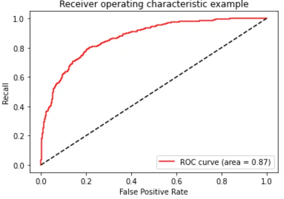
##要想让AUC面积更进一步,我们需要绘制ROC曲线,查看我们是否可以通过调整阈值来对这个模型进行改进。from sklearn.metrics import roc_curve as ROCimport matplotlib.pyplot as pltFPR, Recall, thresholds = ROC(Ytest,clf.decision_function(Xtest),pos_label=1) #(真实值,置信度,正样本是1)area = roc_auc_score(Ytest,clf.decision_function(Xtest))plt.figure()plt.plot(FPR, Recall, color='red',label='ROC curve (area = %0.2f)' % area)plt.plot([0, 1], [0, 1], color='black', linestyle='--')plt.xlim([-0.05, 1.05])plt.ylim([-0.05, 1.05])plt.xlabel('False Positive Rate')plt.ylabel('Recall')plt.title('Receiver operating characteristic example')plt.legend(loc="lower right")plt.show()
以此模型为基础,求解最佳阈值
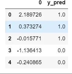
maxindex = (Recall - FPR).tolist().index(max(Recall - FPR)) #先找出插值最大的点的索引thresholds[maxindex] #然后查看这个值#基于我们选出的最佳阈值,我们来认为确定y_predict,并确定在这个阈值下的recall和准确度的值:from sklearn.metrics import accuracy_score as ACtimes = time()clf = SVC(kernel = "linear",C=3.1663157894736838,cache_size = 5000,class_weight = "balanced").fit(Xtrain, Ytrain)prob = pd.DataFrame(clf.decision_function(Xtest))prob.head()prob.loc[prob.iloc[:,0] >= thresholds[maxindex],"y_pred"]=1 #判断>置信度的为1,并添加到y_pred。prob.loc[prob.iloc[:,0] < thresholds[maxindex],"y_pred"]=0prob.head()

若有收获,就点个赞吧
0 人点赞
