K-means聚类
实现K-means
寻找最近中心
def find_closest_centroids(x, centroids):# Set k,初始化中心的行数就是聚类个数k = centroids.shape[0]m = x.shape[0]# You need to return the following variables correctly.idx = np.zeros((m, 1), dtype=np.int32)for i in range(m):idx[i] = 1# 计算当前第i个样本到第一个聚类中心的距离,作为初始化值min_distance = np.linalg.norm(x[i, :] - centroids[1 - 1, :]) ** 2for j in range(2, k + 1):distance = np.linalg.norm(x[i, :] - centroids[j - 1, :]) ** 2if distance < min_distance:min_distance = distanceidx[i] = jreturn idx
更新聚类中心
def compute_centroids(x, idx, k):# Useful variablesm, n = x.shapecentroids = np.zeros((k, n))idx = np.ravel(idx)for i in range(k):centroids[i] = np.mean(x[np.where(idx == i + 1)], axis=0)return centroids
示例数据集上运行K-means
def run_k_means(x, initial_centroids, max_iters, plot_progress=False):if plot_progress:plt.ion()plt.figure()centroids = initial_centroidsprevious_centroids = centroidsk = initial_centroids.shape[0]idx = 0for i in range(max_iters):# Output progressprint('K-Means iteration {}/{}...\n'.format(i + 1, max_iters), flush=True)# For each example in X, assign it to the closest centroididx = find_closest_centroids(x, centroids)# Optionally, plot progress hereif plot_progress:plot_progressk_means(x, centroids, previous_centroids, idx, k, i)previous_centroids = centroids# Given the memberships, compute new centroidscentroids = compute_centroids(x, idx, k)if plot_progress:plt.close()return centroids, idx
图像压缩
print('\nRunning K-Means clustering on pixels from an image.\n\n')A = imread('./data/bird_small.png')# If imread does not work for you, you can try instead# load_mat_file ('bird_small.mat');A = A / 255 # Divide by 255 so that all values are in the range 0 - 1# Size of the imageimg_size = A.shape# Reshape the image into an Nx3 matrix where N = number of pixels.# Each row will contain the Red, Green and Blue pixel values# This gives us our dataset matrix X that we will use K-Means on.X = np.reshape(A, (img_size[0] * img_size[1], 3), order='F')# Run your K-Means algorithm on this data# You should try different values of K and max_iters hereK = 16pixels_iters = 10# When using K-Means, it is important the initialize the centroids# randomly.# You should complete the code in kMeansInitCentroids.m before proceedinginitial_centroids = k_means_init_centroids(X, K)# Run K-Meanscentroids_img, idx_img = run_k_means(X, initial_centroids, pixels_iters)print('Program paused. Press enter to continue.\n')# pause_func()# ================= Part 5: Image Compression ======================print('\nApplying K-Means to compress an image.\n\n')# Find closest cluster membersidx_img_2 = find_closest_centroids(X, centroids_img)X_recovered = np.zeros((idx_img_2.shape[0], X.shape[1]))for i in range(idx_img_2.shape[0]):X_recovered[i] = centroids_img[idx_img_2[i] - 1]X_recovered = np.reshape(X_recovered, (img_size[0], img_size[1], 3), order='F')plt.figure()plt.ion()plt.subplot(121)plt.imshow(A)plt.title('Original')plt.subplot(122)plt.imshow(X_recovered)plt.title('Compressed, with {} colors.'.format(K))plt.pause(5)
PCA(主成分分析)
示例数据集
print('Visualizing example dataset for PCA.\n\n')data = load_mat_file('./data/ex7data1.mat')X = data['X']# Visualize the example datasetplt.ion()plt.figure()# X[:,0]表示取X的每一行的第0列plt.scatter(X[:, 0], X[:, 1])# plt.axis([0.5, 6.5, 2, 8])# 作图为正方形,并且x,y轴范围相同plt.axis("square")plt.pause(0.8)print('Program paused. Press enter to continue.\n')
实现PCA
特征缩放
def feature_normalize(x):x_norm = np.zeros(x.shape)# axis=0,沿列方向计算每行的均值,x输入为50行2列,输出为1行两列mu = np.mean(x, axis=0)sigma = np.std(x, axis=0, ddof=1)for i in range(np.shape(x)[0]):x_norm[i] = (x[i] - mu) / sigmareturn x_norm, mu, sigma
PCA核心
# =============== Part 2: Principal Component Analysis ===============
    print('\nRunning PCA on example dataset.\n\n')
    # Before running PCA, it is important to first normalize X
    X_norm, mu, sigma = feature_normalize(X)
    U, S = pca(X_norm)
    # Draw the eigenvectors centered at mean of data.
    # These lines show the directions of maximum variations in the dataset.
    # 仅仅展示了最大方向
    # 画一条黑色硬实线

    draw_line(mu, (mu + 1.5 * np.dot(S[0], U[:, 0].T)), "-k")
    draw_line(mu, (mu + 1.5 * np.dot(S[1], U[:, 1].T)), "-k")

    plt.pause(0.8)
    print('Top eigenvector: \n')
    print(' U(:,1) = %s \n' % U[:, 0])
    print('\n(you should expect to see -0.707107 -0.707107)\n')

    print('Program paused. Press enter to continue.\n')
    # pause_func()
def pca(x):
    m = x.shape[0]
    # 计算协方差矩阵
    sigma = (1 / m) * (np.dot(x.T, x))
    # 奇异值分解,u为特征向量,s为对角矩阵
    u, s, v = np.linalg.svd(sigma)
    return u, s
投影与重现数据
def project_data(x, u, k):
    k_list = list(range(0, k))
    u_reduce = u[:, k_list]
    return np.dot(x, u_reduce)
def recover_data(z, u, k):
    k_list = list(range(0, k))
    u_reduce = u[:, k_list]
    return np.dot(z, u_reduce.T)
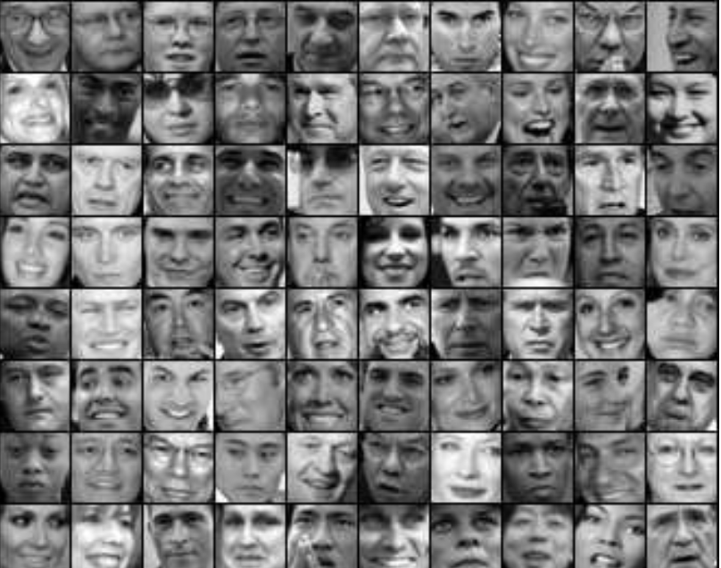
面部数据集
    face_date = load_mat_file('./data/ex7faces.mat')
    X = face_date['X']
    plt.close()
    plt.figure()
    display_data(X[0: 100, :])
    print('Program paused. Press enter to continue.\n')
    # pause_func()

    # =========== Part 5: PCA on Face Data: Eigenfaces  ===================
    # Run PCA and visualize the eigenvectors which are in this case eigenfaces
    # We display the first 36 eigenfaces.
    print('\nRunning PCA on face dataset.\n(this might take a minute or two ...)\n\n')
    # Before running PCA, it is important to first normalize X by subtracting
    # the mean value from each feature
    X_norm, mu, sigma = feature_normalize(X)

    # Run PCA
    U, S = pca(X_norm)
    # Visualize the top 36 eigenvectors found
    plt.close()
    plt.figure()
    display_data(U[:, 0:36].T)
    print('Program paused. Press enter to continue.\n')
    # pause_func()

    # ============= Part 6: Dimension Reduction for Faces =================
    # Project images to the eigen space using the top k eigenvectors
    # If you are applying a machine learning algorithm
    print('\nDimension reduction for face dataset.\n\n')

    K = 100
    Z = project_data(X_norm, U, K)

    print('The projected data Z has a size of: ')
    print(Z.shape)

    print('Program paused. Press enter to continue.\n')
    # pause_func()

    # ==== Part 7: Visualization of Faces after PCA Dimension Reduction ====
    # Project images to the eigen space using the top K eigen vectors and
    # visualize only using those K dimensions
    # Compare to the original input, which is also displayed

    print('\nVisualizing the projected (reduced dimension) faces.\n\n')
    K = 100
    X_rec = recover_data(Z, U, K)
    # Display normalized data
    plt.close()
    plt.figure()
    plt.subplot(1, 2, 1)
    plt.title('Original faces')
    display_data(X_norm[0:100, :])

    # Display reconstructed data from only k eigenfaces
    plt.subplot(1, 2, 2)
    plt.title('Recovered faces')
    display_data(X_rec[0:100, :])
    plt.close()

    print('Program paused. Press enter to continue.\n')

若有收获,就点个赞吧
0 人点赞
