背景
1. 正则化线性回归
1.1 可视化数据集
plt.ion()#返回单张图像plt.figure()#直接输出,不阻塞plt.plot(X, y, 'rx', markersize=10)plt.xlabel('Change in water level (x)')plt.ylabel('Water flowing out of the dam (y)')plt.axis([-60, 40, 0, 40])plt.pause(2)plt.close()
pyplot.ion:
在使用matplotlib的过程中,常常会需要画很多图,但是好像并不能同时展示许多图。这是因为python可视化库matplotlib的显示模式默认为阻塞(block)模式。什么是阻塞模式那?我的理解就是在plt.show()之后,程序会暂停到那儿,并不会继续执行下去。如果需要继续执行程序,就要关闭图片。那如何展示动态图或多个窗口呢?这就要使用plt.ion()这个函数,使matplotlib的显示模式转换为交互(interactive)模式。即使在脚本中遇到plt.show(),代码还是会继续执行。
- 在交互模式下:
- plt.plot(x)或plt.imshow(x)是直接出图像,不需要plt.show()
- 如果在脚本中使用ion()命令开启了交互模式,没有使用ioff()关闭的话,则图像会一闪而过,并不会常留。要想防止这种情况,需要在plt.show()之前加上ioff()命令。
- 在阻塞模式下:
- 打开一个窗口以后必须关掉才能打开下一个新的窗口。这种情况下,默认是不能像Matlab一样同时开很多窗口进行对比的。
- plt.plot(x)或plt.imshow(x)是直接出图像,需要plt.show()后才能显示图像

1.2 正则化线性回归损失函数

def linear_reg_cost_function(x, y, theta, linear_lambda):theta = np.reshape(theta, (theta.shape[0], 1))m = x.shape[0]h = np.dot(x, theta)j_without_regularization = (1 / (2 * m)) * np.sum((h - y) ** 2)j = j_without_regularization + (linear_lambda / (2 * m)) * np.sum(theta[1:] ** 2)grad_without_regularization = (np.dot(x.T, h - y) / m)grad = grad_without_regularization + (linear_lambda / m) * thetagrad[0] = grad_without_regularization[0]return j, grad
1.3 正则化线性回归梯度下降公式

 的索引。
的索引。
1.4 拟合线性回归
pyplot.plot函数
https://blog.csdn.net/sinat_36219858/article/details/79800460
def train_linear_reg(x, y, train_lambda):initial_theta = np.zeros((x.shape[1], 1))global gradgrad = np.zeros((x.shape[1], 1))return sciopt.minimize(fun=cost_function, x0=initial_theta, args=(x, y, train_lambda), method="TNC", jac=gradient)def cost_function(theta, x, y, cf_lambad):j, new_grad = linear_reg_cost_function(x, y, theta, cf_lambad)global gradgrad = new_gradreturn jdef gradient(*args):global gradreturn grad.flatten()
2. 偏差方差
def learning_curve(x, y, xval, yval, curve_lambda):m = x.shape[0]m_xval = xval.shape[0]error_train = np.zeros((m, 1))error_val = np.zeros((m, 1))x = np.append(np.ones((m, 1)), x, axis=1)xval = np.append(np.ones((m_xval, 1)), xval, axis=1)for i in range(m):# compute parameter thetaresult = train_linear_reg(x[0:i + 1], y[0:i + 1], curve_lambda)theta = result['x']# compute training errorerror_train[i] = linear_reg_cost_function(x[0:i + 1], y[0:i + 1], theta, 0)[0]# compute cross validation errorerror_val[i] = linear_reg_cost_function(xval, yval, theta, 0)[0]return error_train, error_val
3. 多项式回归
3.1 特征映射
def poly_features(x, p):m = x.shape[0]x_poly = np.zeros((m, p))for i in range(p):x_poly[:, i] = (x ** (i + 1)).reshape(m, )return x_polydef feature_normalize(x):x_norm = np.zeros(x.shape)mu = np.mean(x, axis=0)sigma = np.std(x, axis=0, ddof=1)for i in range(np.shape(x)[0]):x_norm[i] = (x[i] - mu) / sigmareturn x_norm, mu, sigma
3.2 学习多项式回归
lc_pr_lambda = 1theta = train_linear_reg(X_poly, y, lc_pr_lambda)['x']# Plot training data and fitplt.figure()plt.plot(X, y, 'rx', markersize=10)plot_fit(np.min(X), np.max(X), mu, sigma, theta, p)plt.xlabel('Change in water level (x)')plt.ylabel('Water flowing out of the dam (y)')plt.title('Polynomial Regression Fit (lambda = %f)' % lc_pr_lambda)plt.pause(2)plt.close()error_train, error_val = learning_curve(X_poly, y, X_poly_val, yval, lc_pr_lambda)plt.figure()plt.plot(np.arange(m), error_train)plt.plot(np.arange(m), error_val)plt.title('Polynomial Regression Learning Curve (lambda = %f)' % lc_pr_lambda)plt.xlabel('Number of training examples')plt.ylabel('Error')plt.legend(['Train', 'Cross Validation'])
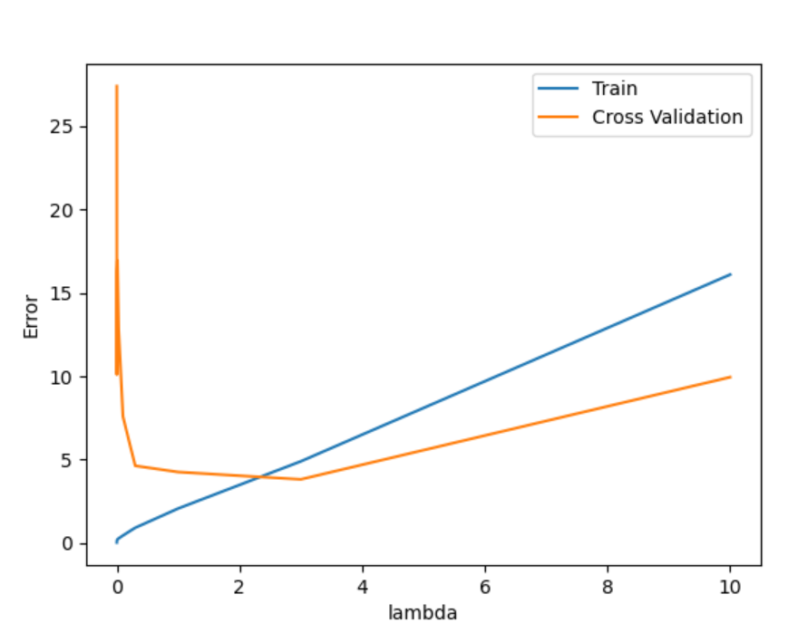
3.3 不同的lamda
def validation_curve(x, y, xval, yval):# Selected values of lambda (you should not change this)lambda_vec = np.array(([0, 0.001, 0.003, 0.01, 0.03, 0.1, 0.3, 1, 3, 10]))len_of_vec = len(lambda_vec)# You need to return these variables correctly.error_train = np.zeros((len_of_vec, 1))error_val = np.zeros((len_of_vec, 1))for i in range(len_of_vec):lambda_temp = lambda_vec[i]# compute parameter theta (learning)result = train_linear_reg(x, y, lambda_temp)theta = result['x']# compute training errorj, grad = linear_reg_cost_function(x, y, theta, 0)error_train[i] = j# compute cross validation errorj, grad = linear_reg_cost_function(xval, yval, theta, 0)error_val[i] = jreturn lambda_vec, error_train, error_val

若有收获,就点个赞吧
0 人点赞
