1.函数

# coding=gbkimport numpy as npimport matplotlib.pyplot as pltfrom scipy import signalplt.rcParams['figure.figsize'] = (8, 4.5) # 设置figure_size尺寸plt.rcParams['figure.dpi'] = 150 # 分辨率plt.rcParams['savefig.dpi'] = 300 # 图片像素plt.rcParams['image.interpolation'] = 'nearest' # 设置 interpolation styleplt.rcParams['image.cmap'] = 'gray' # 设置 颜色 style# 默认的像素:[6.0,4.0],分辨率为100,图片尺寸为 600&400# 指定dpi=200,图片尺寸为 1200*800# 指定dpi=300,图片尺寸为 1800*1200# 设置figsize可以在不改变分辨率情况下改变比例x1 = np.linspace(-5, 5, 10000)y1 = x1 - np.sin(x1)plt.plot(x1, y1, c = 'k', label = r"$ y=x-sinx $")plt.grid()plt.legend()plt.show()


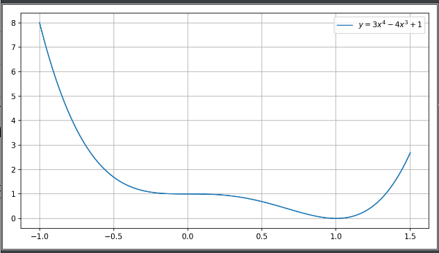
x1 = np.linspace(-1, 1.5, 1000)
y1 = 3 * (x1 ** 4) - 4 * (x1 ** 3) + 1
plt.plot(x1, y1, label = r"$ y = 3x^4 - 4x^3 + 1 $")

a = 1
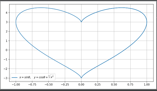
theta = np.arange(0, 2 * np.pi, np.pi / 180)
x = np.sin(theta)
y = 3*np.cos(theta) + 3*np.power((x ** 2), 1 / 3) # 原来用 y = np.cos(theta) + np.power(x, 2/3)只画出一半,而且报power的错
plt.plot(x, y, label=r'$x=sin\theta,\quady=cos\theta+\sqrt[3]{x^2}$')
plt.grid('equal')
plt.legend()
plt.show()
x = np.linspace(0, 10, 1000) #自变量
y = np.sin(x) + 1
z = np.cos(x**2) + 1

plt.plot(x, y, label='\$sin x+1$', color='red', linewidth='2')  # 作图,设置标签,线条颜色,大小
plt.plot(x, z, 'b--', label='\cos x^2+1')
plt.xlabel('Time(s)')  # x轴名称
plt.ylabel('Vlot')  # y轴名称
plt.title('A Simple Example')  # 标题
plt.xlim(0, 10)  # x轴范围
plt.ylim(0, 2.2)  # y轴范围
plt.legend()  # 显示图例
plt.show()  # 显示作图结果


若有收获,就点个赞吧
0 人点赞
