2.1 Model Representation

模型描述
To establish notation for future use, we’ll use to denote the “input” variables (living area in this example), also called input features,
我们定义一些符号方便将来使用，我们将用 来表示“输入”变量 (本示例为居住区域)，也称为输入特征

and to denote the “output” or target variable that we are trying to predict (price).
并且用来表示“输出”变量 或者 我们试图预测的目标变量（价格）。

A pair is called a training example, and the dataset that we’ll be using to learn—a list of m training examples ; i=1,…,m— is called a training set.
一对被称为训练样本，以及我们将用来学习的数据集-m个训练示例的列表； i = 1，…，m-称为训练集。

Note that the superscript “(i)” in the notation is simply an index into the training set, and has nothing to do with exponentiation.
注意，符号中的上标 “(i)” 只是训练集中的一个索引，与幂运算无关。

We will also use X to denote the space of input values, and Y to denote the space of output values. In this example, X = Y = ℝ.
我们还将使用X表示输入值的空间，并使用Y表示输出值的空间。 在此示例中，X = Y =ℝ。

To describe the supervised learning problem slightly more formally, our goal is, given a training set, to learn a function h : X → Y so that h(x) is a “good” predictor for the corresponding value of y.
为了更正式地描述监督学习问题，我们的目标是给定训练集，以学习函数h：X→Y，以便 h(x) 是y对应值的“良好”预测因子。

For historical reasons, this function h is called a hypothesis. Seen pictorially, the process is therefore like this:
由于历史原因，这个函数h被称为假设。从图片上看，这个过程是这样的: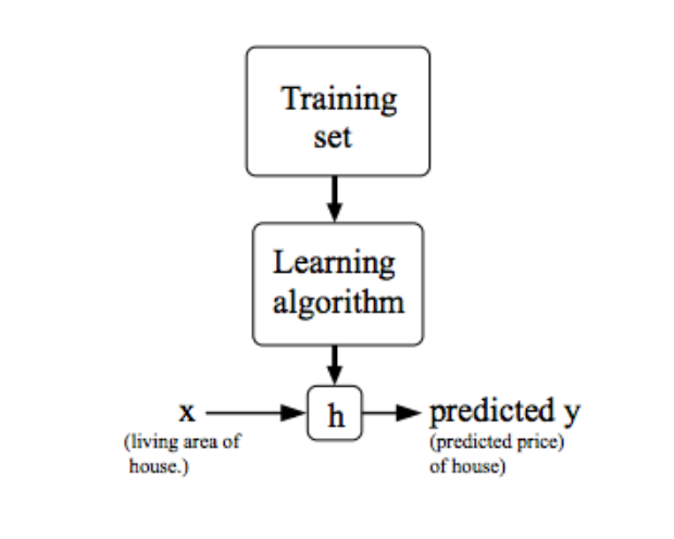

When the target variable that we’re trying to predict is continuous, such as in our housing example, we call the learning problem a regression problem.
当我们要预测的目标变量是连续的时（例如在我们的住房示例中），我们将学习问题称为回归问题。

When y can take on only a small number of discrete values (such as if, given the living area, we wanted to predict if a dwelling is a house or an apartment, say), we call it a classification problem.
当y只能采用少量离散值时（例如，假设给定居住面积，我们想预测某个住宅是房子还是公寓），我们称其为分类问题。

2.2 Cost Function

代价函数
We can measure the accuracy of our hypothesis function by using a cost function.
我们可以使用代价函数来衡量假设函数的准确性。
This takes an average difference (actually a fancier version of an average) of all the results of the hypothesis with inputs from x’s and the actual output y’s.
这将 假设的所有结果 与 x的输入 和 实际输出y 的 平均值进行平均差（实际上是平均值的简化形式）。

This function is otherwise called the “Squared error function”, or “Mean squared error”.
这个函数也被称为“平方误差函数”或“平均平方误差”。

The mean is halved 1/2 as a convenience for the computation of the gradient descent, as the derivative term of the square function will cancel out the 1/2 term.
平均值减半是为了方便梯度下降的计算，因为平方函数的导数项会抵消1/2项。
The following image summarizes what the cost function does:
下图总结了代价函数的作用：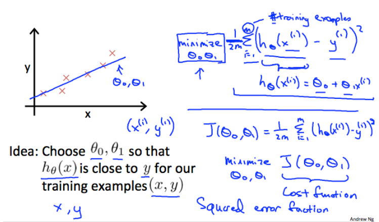

2.3 Cost Function - Intuition I

If we try to think of it in visual terms, our training data set is scattered on the x-y plane.
如果我们尝试从视觉上考虑它，我们的训练数据集将散布在x-y平面上。

We are trying to make a straight line (defined by ) which passes through these scattered data points.
我们正在尝试使一条直线（由定义）穿过这些分散的数据点。

Our objective is to get the best possible line.
我们的目标是获得最佳可能的线。

The best possible line will be such so that the average squared vertical distances of the scattered points from the line will be the least.
最佳可能的线应该使散射点与该线的平均垂直垂直距离最小。
Ideally, the line should pass through all the points of our training data set.
理想情况下，直线应穿过训练数据集中的所有点。
In such a case, the value of will be 0. The following example shows the ideal situation where we have a cost function of 0.
在这种情况下，的值将为0。下例显示了代价函数为0的理想情况。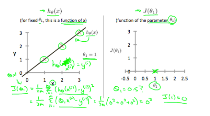

When , we get a slope of 1 which goes through every single data point in our model.
当时，我们得到的斜率为1的直线，该直线贯穿模型中的每个数据点。
Conversely, when , we see the vertical distance from our fit to the data points increase.
相反，当时，我们看到拟合直线到数据点的垂直距离增加。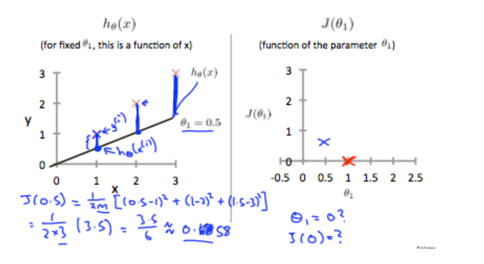

This increases our cost function to 0.58. Plotting several other points yields to the following graph:
当代价函数提高到0.58。 绘制其他几个点可得出下图：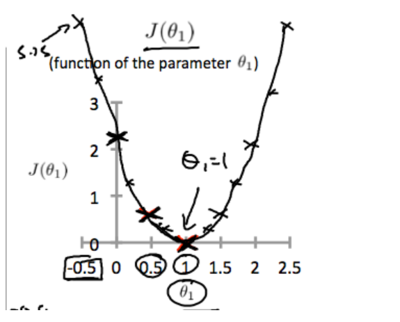

Thus as a goal, we should try to minimize the cost function. In this case, is our global minimum.
因此，我们的目标为应尽量降低代价函数的值。 在这种情况下， 是我们的总体的最小值。

2.4 Cost Function - Intuition II

A contour plot is a graph that contains many contour lines.
等高线图是包含许多等高线的图形。

A contour line of a two variable function has a constant value at all points of the same line.
两个变量函数的轮廓线在同一条线的所有点上均具有恒定值。

An example of such a graph is the one to the right below.
这种图的一个示例是下面的右图。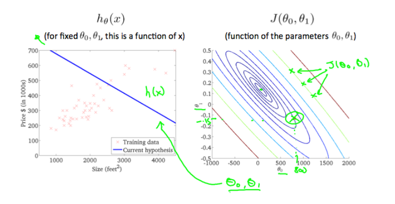

Taking any color and going along the ‘circle’, one would expect to get the same value of the cost function.
采用任何颜色并沿“圆”移动，我们都会得到与代价函数相同的值。

For example, the three green points found on the green line above have the same value for and as a result, they are found along the same line.
例如，在上面的绿线上找到的三个绿点在上具有相同的值，因此，它们在同一条线上找到。

The circled x displays the value of the cost function for the graph on the left when and .
带圆圈的x在和时在左侧显示图形的代价函数的值当 , 。

Taking another h(x) and plotting its contour plot, one gets the following graphs:
取另一个h(x)并绘制其等值线图，得到如下图: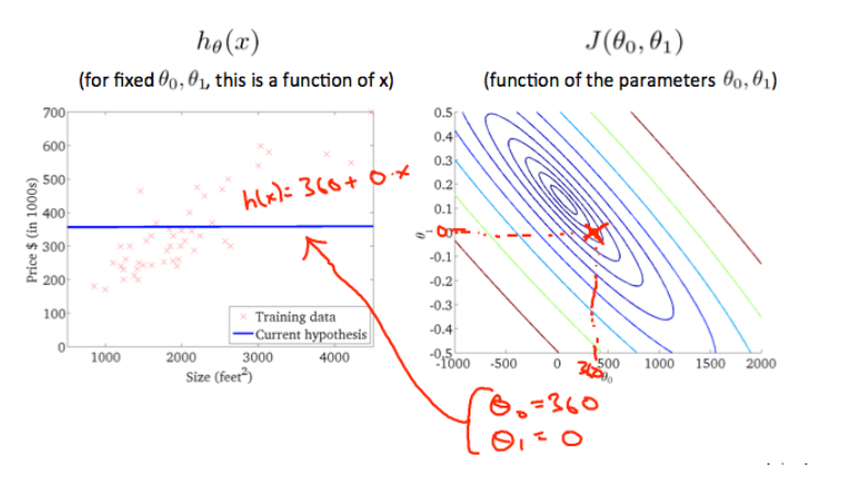

When and , the value of in the contour plot gets closer to the center thus reducing the cost function error.
当 且 时，等高线图中的值更接近中心，从而减少了代价函数误差。

Now giving our hypothesis function a slightly positive slope results in a better fit of the data.
现在给我们的假设函数一个稍微为正的斜率，可以更好地拟合数据。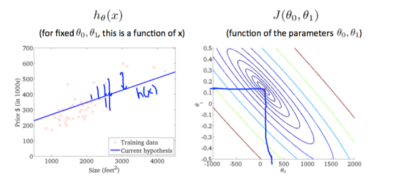

The graph above minimizes the cost function as much as possible and consequently, the result of and tend to be around 0.12 and 250 respectively.
上面的图表尽可能地使代价函数最小化，因此， 和 结果和分别约为0.12和250。
Plotting those values on our graph to the right seems to put our point in the center of the inner most ‘circle’.
将图形上的值绘制到右侧似乎使我们的点处于最内部的“圆”的中心。