pandaspython
由于numpy 对于元素类别的限制(必须得是同一类型元素),因此在存储多种类别信息时,就显得有些捉襟见肘了。
而pandas,则应运而生。其存储数据格式,非常类似于R中的data_frame。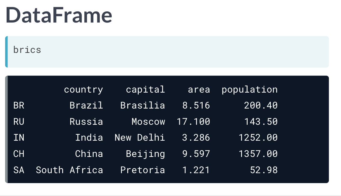
pandas
构建dataframe
1)构建字典example_dict,字典值为键信息所对应的列表。
2)将构建的字典转化为pandas包中的dataframe形式。example = pd.DataFrame(example_dict)。
也可以通过导入外部文件的方式,如example = pd.read_csv('example.csv')
3)若外部文件中不包含行注释,可以为dataframe 构建标签,example.index = row_labels。若引入的文件本身包含row_labels,则在导入文件时需要增加选项index_col = 0,否则pandas 会默认为表格添加一行注释。
import pandas as pd# Build cars DataFramenames = ['United States', 'Australia', 'Japan', 'India', 'Russia', 'Morocco', 'Egypt']dr = [True, False, False, False, True, True, True]cpc = [809, 731, 588, 18, 200, 70, 45]cars_dict = { 'country':names, 'drives_right':dr, 'cars_per_cap':cpc }cars = pd.DataFrame(cars_dict)print(cars)# Definition of row_labelsrow_labels = ['US', 'AUS', 'JPN', 'IN', 'RU', 'MOR', 'EG']# Specify row labels of carscars.index = row_labels# Print cars againprint(cars)
ps:另外,还有一种构建dataframe 的思路,也就是建造包含许多字典的列表(先前是每个键对应列表的字典)。也就是一行一行的添加,因为每次都必须输入重复的键,所以这种方式比较繁琐。
快速查看dataframe
*.head() ,输出图表前几行信息。*.info() ,输出图表列信息,数量、类型、空间占用等。*.shape() ,输出图表row x col 信息。*.describe() ,输出图表数据的一些统计学计算结果。
# 如“homelessness”数据集的describe 返回结果。
        individuals  family_members  state_pop
    count       51.000          51.000  5.100e+01
    mean      7225.784        3504.882  6.406e+06
    std      15991.025        7805.412  7.327e+06
    min        434.000          75.000  5.776e+05
    25%       1446.500         592.000  1.777e+06
    50%       3082.000        1482.000  4.461e+06
    75%       6781.500        3196.000  7.341e+06
    max     109008.000       52070.000  3.946e+07
*.values ,输出二维numpy列表,包含原来图表每一行的信息。*.columns ,指引出图表中全部列名称。*.index ,指引出图表中全部行信息,数字或名称。
选择dataframe 中的信息
data_frame[] 会生成一个panda_series 类型内容。
而如果想将结果返回为dataframe,需要使用双方括号,data_frame[[]]。
data_frame 也是支持切片操作的,且列使用名称,行使用且仅使用切片。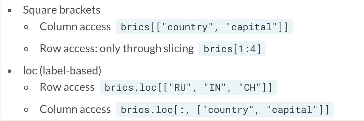
loc 与iloc
data_frame.loc[],通过向其中输入列表,[row_label_dict, col_label_dict],从而指定输出选择的行与列的信息。
通常来说, ix 可与 iloc 有相似的功能。
iloc 与loc 一样,只不过由名称选择变成了位置选择。另外loc 和一般切片不同,是包含选择的前后内容的,而iloc 符合一般切片规则,“包头不包尾”。
# Import cars data
import pandas as pd
cars = pd.read_csv('cars.csv', index_col = 0)

# Print out drives_right column as Series
print(cars.iloc[:, 2])

# Print out drives_right column as DataFrame
print(cars.iloc[:, [2]])

# Print out cars_per_cap and drives_right as DataFrame
print(cars.loc[:, ['cars_per_cap', 'drives_right']])
使用比较运算符进行筛选
# Import cars data
import pandas as pd
cars = pd.read_csv('cars.csv', index_col = 0)

# Create car_maniac: observations that have a cars_per_cap over 500
cpc = cars['cars_per_cap']
many_cars = cpc > 500 # 返回布尔值
car_maniac = cars[many_cars] # 只返回True 的row

# Print car_maniac
print(car_maniac)
- 还可以结合numpy 结合and, or, not 这些比较字符,实现更高效的筛选。
# Import cars data
import pandas as pd
cars = pd.read_csv('cars.csv', index_col = 0)

# Import numpy, you'll need this
import numpy as np

# Create medium: observations with cars_per_cap between 100 and 500
medium = cars[np.logical_and(cars['cars_per_cap'] > 100, cars['cars_per_cap'] < 500)]


# Print medium
print(medium)
当然上式中的medium 也可以利用其他操作子实现。
medium = cars[(cars['cars_per_cap'] > 100) & (cars['cars_per_cap'] < 500)]
& 表示 and,| 表示 or。
query
query 更加简单粗暴。用于条件筛选符合条件行内容。
medium = cars.query("cars_per_cap > 100 & cars_per_cap < 500")
isin
当如果选择符合某列中的多行信息的内容时,如果单一的使用 操作子 或者 logical_and 方法,会非常的繁琐。isin 提供了一个非常好的选择。df[df["col"].isin(["value_1", "value_2"])]
# The Mojave Desert states
canu = ["California", "Arizona", "Nevada", "Utah"]

# Filter for rows in the Mojave Desert states
mojave_homelessness = homelessness[homelessness["state"].isin(canu)]

# See the result
print(mojave_homelessness)
创建索引
我们可以通过将dataframe 中的col 从主体中移出,将其设定为index。test_index = test.set_index('col_index')
如果想要移出添加的索引, test_index.reset_index() 。索引就会回到表格主体。如果设定参数 drop=True ,则索引会被直接删除。
通过创建索引,可以让我们的列表提取操作更加方便。
df[df["col"].isin(["value_1", "value_2"])] ,可以提取目标col 中包含选定值的内容。但如果构建了索引,则更加方便。df_ind = df.set_index('col') ,接着就可以直接通过loc 选择目标行名称, df_ind.loc[['val_1', 'val_2']] 。
另外,也可以通过列表,将多列同时选定为索引,其中先选择的列为外部索引,后选择的列为内部索引。
如果想要传入一组index,即同时选中index 的两个信息,需要将内容以元组的形式在列表中输入。test_index.loc[[('val1_1', 'val2_1'), ('val1_2', 'val2_2')]] 。
# Index temperatures by country & city
temperatures_ind = temperatures.set_index(['country', 'city'])

# List of tuples: Brazil, Rio De Janeiro & Pakistan, Lahore
rows_to_keep = [('Brazil', 'Rio De Janeiro'), ('Pakistan', 'Lahore')]

# Subset for rows to keep
print(temperatures_ind.loc[rows_to_keep])
还可以重新设定索引顺序, .reindex(list_with_desired_order) 。当reindex 的内容中有不存在的label时,对应的行信息会显示为NaN。因此这也可以用来找寻两个表格的相同index信息。
# Import pandas
import pandas as pd

# Reindex names_1981 with index of names_1881: common_names
common_names = names_1981.reindex(names_1881.index)

# Print shape of common_names
print(common_names.shape)

# Drop rows with null counts: common_names
common_names = common_names.dropna()

# Print shape of new common_names
print(common_names.shape)

'''
Shape of names_1981 DataFrame: (19455, 1)
Shape of names_1881 DataFrame: (1935, 1)

<script.py> output:
    (1935, 1)
    (1587, 1)
'''
也可以利用index 进行排序, test_index.sort_index() ,默认由外部索引到内部索引,按照升序排列。
# Sort temperatures_ind by index values
print(temperatures_ind.sort_index())

# Sort temperatures_ind by index values at the city level
print(temperatures_ind.sort_index(level="city"))

# Sort temperatures_ind by country then descending city
print(temperatures_ind.sort_index(level=["country", "city"], ascending = [True, False]))
index 中的切片操作
index 无法对内部index 进行直接操作,否则会返回一个空表(但它不会报错的!!)。正确的做法是将字符串替换为元组,两边元组包含外部index 与内部index 的开头以及它们的结尾。
如果想要对内部index 进行操作,需要借助 pd.IndexSilce 函数。
.loc[pd.IndexSlice[:,'inner_index'], :])

.loc[:, pd.IndexSlice[:, 'inner_index']]
另外还可以进行两次切片操作,先对index操作,再对列进行操作。
且使用loc 对index 进行操作,可以输入信息部分内容,对其进行选择。
# Use Boolean conditions to subset temperatures for rows in 2010 and 2011
temperatures_bool = temperatures[(temperatures["date"] >= "2010-01-01") & (temperatures["date"] <= "2011-12-31")]
print(temperatures_bool)

# Set date as an index
temperatures_ind = temperatures.set_index("date")

# Use .loc[] to subset temperatures_ind for rows in 2010 and 2011
print(temperatures_ind.loc["2010":"2011"])

# Use .loc[] to subset temperatures_ind for rows from Aug 2010 to Feb 2011
print(temperatures_ind.loc["2010-08":"2011-02"])
index 的整理
.resample('A') ,可以将index 的内容进行排序,A表示年。.resample('').last() ,结合last 后可以选中resample后最后输出的几个元素。
index 的问题

整理dataframe
排序
*.sort_values() ,默认按照升序排列,可以自行修改,增加参数选项, ascending ,True 为默认,表升序,False 表降序。
去重
.drop_duplicates(subset='col') ,可以去除指定列中重复的项,返回一个各行中指定列数据均唯一的表格。也可以给subset 指定一个表格,这样可以对多列进行去重,只有多列的信息完全一致时才会舍去。
修改
.str.replace('F', 'C') ,可以将本来表格中的F 替换为C。
.multiply() 用于计算乘法。可以指定其中为表格相关类型的数据,并设定axis 参数,按照行或列进行计算,将元素数据进行替换。
# Import pandas
import pandas as pd

# Read 'sp500.csv' into a DataFrame: sp500
sp500 = pd.read_csv('sp500.csv', index_col = 'Date', parse_dates=True)

# Read 'exchange.csv' into a DataFrame: exchange
exchange = pd.read_csv('exchange.csv', index_col = 'Date', parse_dates=True)

# Subset 'Open' & 'Close' columns from sp500: dollars
dollars = sp500[['Open', 'Close']]

# Print the head of dollars
print(dollars.head())

# Convert dollars to pounds: pounds
pounds = dollars.multiply(exchange['GBP/USD'], axis='rows')

# Print the head of pounds
print(pounds.head())
为dataframe添加新内容
直接添加
比如新行为旧行数字减1, df['new_col'] = df['old_col'] - 1
# Add total col as sum of individuals and family_members
homelessness['total'] = homelessness['individuals'] + homelessness["family_members"]

# Add p_individuals col as proportion of individuals
homelessness['p_individuals'] = homelessness['individuals'] / (homelessness['individuals'] + homelessness["family_members"])

# See the result
print(homelessness)
利用函数添加
利用迭代添加新行
因为dataframe格式文件,从某种意义来说属于2Darray,因此需要用特殊的方法进行遍历。
使用 *.iterrows() 方法。
# Import cars data
import pandas as pd
cars = pd.read_csv('cars.csv', index_col = 0)

# Iterate over rows of cars
for lab, row in cars.iterrows():
    print(lab)
    print(row)
xxx.loc[lab, "COUNTRY"] = row['country'].function()
# Import cars data
import pandas as pd
cars = pd.read_csv('cars.csv', index_col = 0)

# Code for loop that adds COUNTRY column
for lab, row in cars.iterrows() :
    cars.loc[lab, "COUNTRY"] = row["country"].upper()

# Print cars
print(cars)
利用apply 实现添加
# Import cars data
import pandas as pd
cars = pd.read_csv('cars.csv', index_col = 0)

# Use .apply(str.upper)
cars["COUNTRY"] = cars["country"].apply(str.upper)
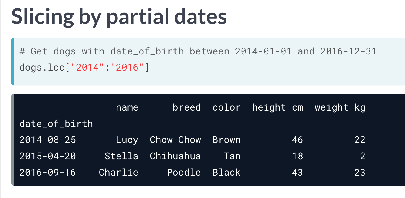
利用函数添加新列
可以使用qcut() 函数。
使用cut() 也可以实现同样效果。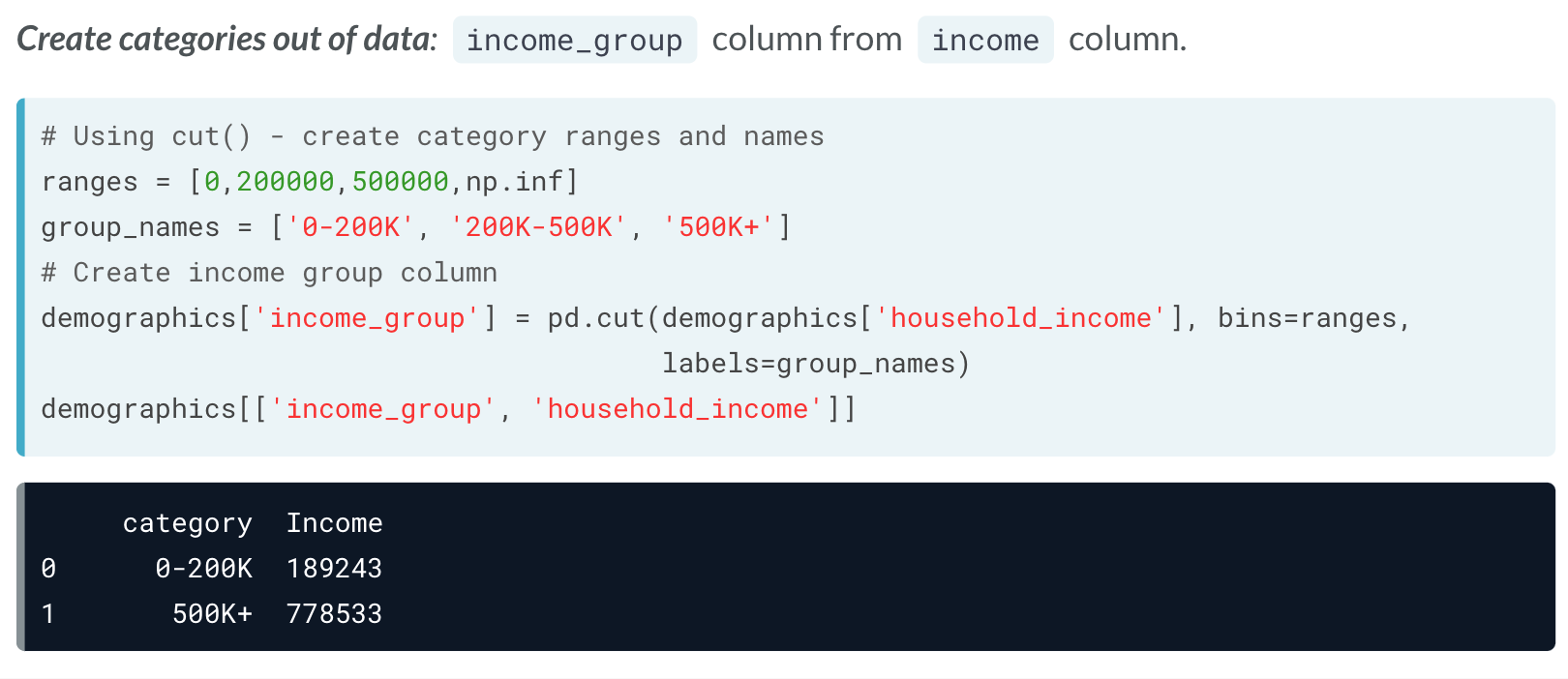
缺失数据
pandas 的dataframe中,缺失值通过 NaN 表示。
查看缺失数据
df.isna() 。将表格中的全部数据以布尔值形式返回,缺失值返回True。但对于大量数据,这样有点儿不方便。df.col.isnull() 则可以查询表格中的特定列中的缺失值。df.isna().any() ,会返回每列是否有缺失值,有缺失值返回True。df.isna().sum() ,返回每列缺失值的总数。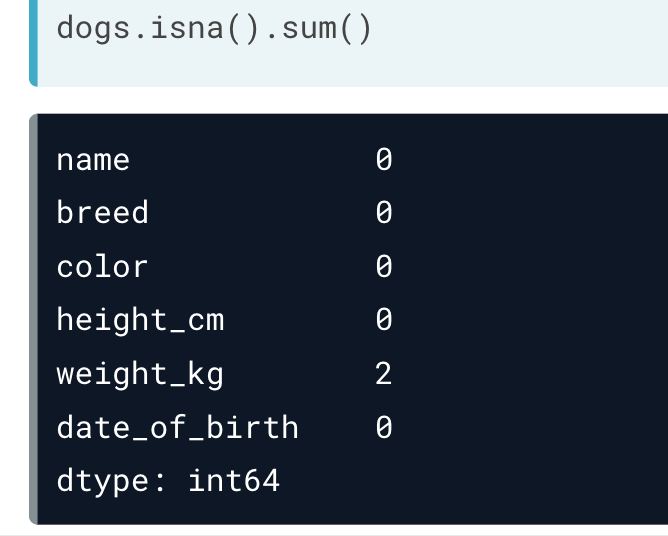
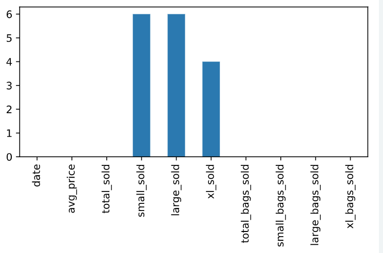
这里还可以联合条形图,图像化显示各组的缺失值信息。
# Bar plot of missing values by variable
avocados_2016.isna().sum().plot(kind = 'bar')

# Show plot
plt.show()
处理缺失数据
df.dropna() ,直接将存在丢失值的一行删去。df.fillna(0) ,将缺失值用0替代。df.ffill() ,会将缺失值向上取值进行替代(最近的一个有数值的行)。
# Import pandas
import pandas as pd

# Reindex weather1 using the list year: weather2
weather2 = weather1.reindex(year)

# Print weather2
print(weather2)

# Reindex weather1 using the list year with forward-fill: weather3
weather3 = weather1.reindex(year).ffill()

# Print weather3
print(weather3)

'''
<script.py> output:
           Mean TemperatureF
    Month
    Jan            32.133333
    Feb                  NaN
    Mar                  NaN
    Apr            61.956044
    May                  NaN
    Jun                  NaN
    Jul            68.934783
    Aug                  NaN
    Sep                  NaN
    Oct            43.434783
    Nov                  NaN
    Dec                  NaN
           Mean TemperatureF
    Month
    Jan            32.133333
    Feb            32.133333
    Mar            32.133333
    Apr            61.956044
    May            61.956044
    Jun            61.956044
    Jul            68.934783
    Aug            68.934783
    Sep            68.934783
    Oct            43.434783
    Nov            43.434783
    Dec            43.434783
'''
统计分析
和numpy 库一样,pandas 也有许多统计学计算的功能。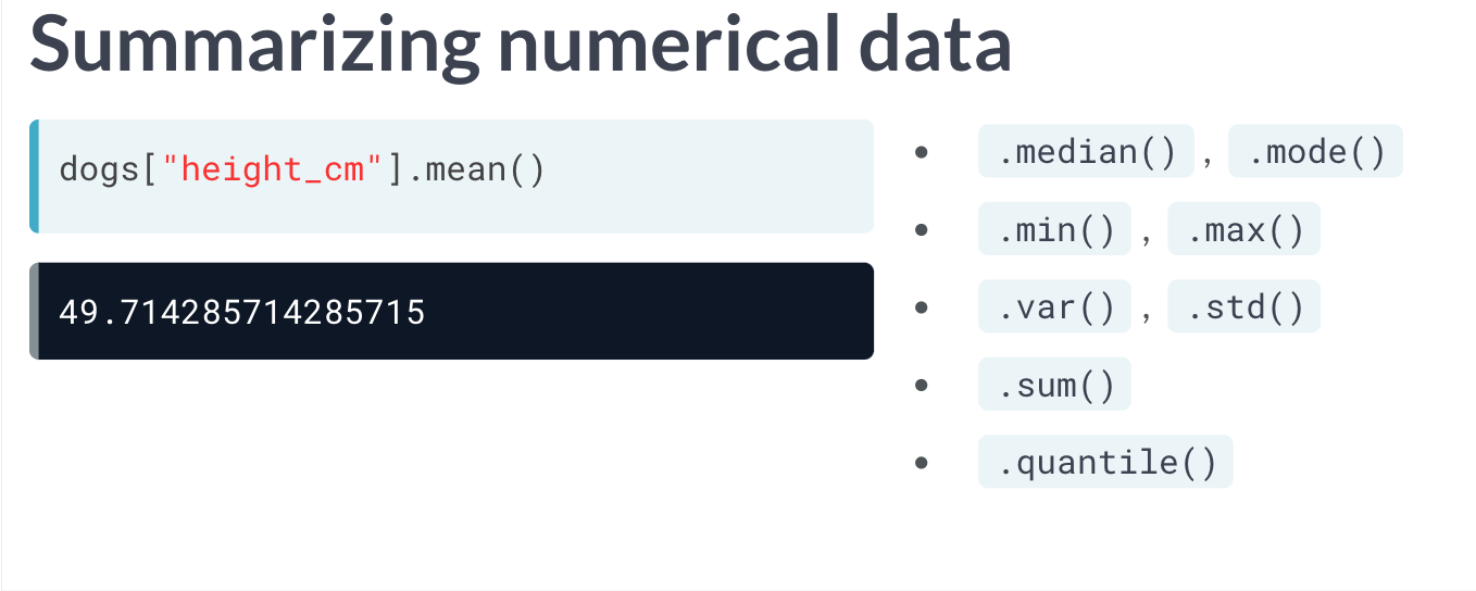
此外, .cum*() 还可以计算每行的累计结果,结果以列的形式返回。如 .cummax() , .cummin() , .cumprod() , .cumsum() 等等。
dataframe.divide(select_frame) 可以将原dataframe 中的数据与选中的数据一一进行对比,并返回一个比值。需要注意的是,二者需要拥有相同的列数和索引。
.agg 方法
.agg() 可以使我们快速计算同一内容的多个统计学相关结果。
比如现在我们的 data_frame 中有一组感兴趣的数据, height_cm ,我们想要计算这组数据的 mean , min ,与 quantile(0.3) 。
我们可以粗暴地一个一个的函数调用。
data_frame['height_cm'].mean()
data_frame['height_cm'].min()
data_frame['height_cm'].quantile(0.3)
但如果我们除了想要知道height_cm,还有weight_kg 的30%的取值,还要知道40%取值时,就可以构造函数及使用agg方便我们批量调用。
def pct40(col):
    return col.quantile(0.4)

def pct30(col):
    return col.quantile(0.3)

data_frame[['height_cm', 'weight_kg']].agg([pcf30, pcf40])
计数
example['col'].value_counts() ,此外还有选项sort(True 为降序), normalize(默认为False)使分组各类别返回为所占的百分比。
# Count the number of stores of each type
store_counts = store_types["type"].value_counts()
print(store_counts)

# Get the proportion of stores of each type
store_props = store_types["type"].value_counts(normalize=True)
print(store_props)

# Count the number of each department number and sort
dept_counts_sorted = store_depts["department"].value_counts(sort=True)
print(dept_counts_sorted)

# Get the proportion of departments of each number and sort
dept_props_sorted = store_depts["department"].value_counts(sort=True, normalize=True)
print(dept_props_sorted)
分组分析
bygroup
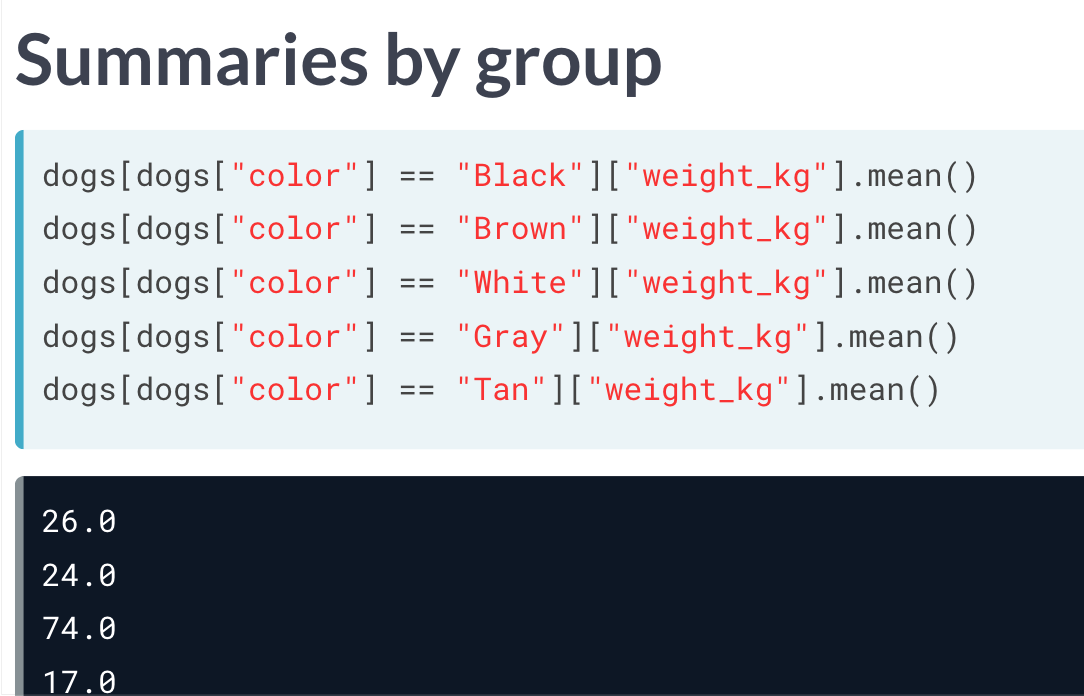
利用先前所学的知识,我们可以利用条件和运算符,对其进行选择,但这未免有些冗杂。
dataframe.groupby('by_col')['col'].mean() ,可以得到同样的结果。
除此之外,我们还可以结合 .agg ,同时获取更多的统计分析结果。dataframe.groupby('by_col')['col'].agg([max, min, mean, sum]) 。而分组的col与统计分析的col 也都可以通过列表一次输入多个进行分析。
# Group by type and is_holiday; calc total weekly sales
sales_by_type_is_holiday = sales.groupby(['type', 'is_holiday'])['weekly_sales'].sum()
print(sales_by_type_is_holiday)

'''
<script.py> output:
    type  is_holiday
    A     False         2.337e+08
          True          2.360e+04
    B     False         2.318e+07
          True          1.621e+03
    Name: weekly_sales, dtype: float64
'''
结合.agg
# Import NumPy with the alias np
import numpy as np

# For each store type, aggregate weekly_sales: get min, max, mean, and median
sales_stats = sales.groupby("type")["weekly_sales"].agg([np.min, np.max, np.mean, np.median])

# Print sales_stats
print(sales_stats)

# For each store type, aggregate unemployment and fuel_price_usd_per_l: get min, max, mean, and median
unemp_fuel_stats = sales.groupby("type")[["unemployment", "fuel_price_usd_per_l"]].agg([np.min, np.max, np.mean, np.median])

# Print unemp_fuel_stats
print(unemp_fuel_stats)
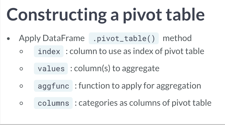
pivot_table
 v
v
相比起bygroup 是筛选原先列表的数据进行分析,pivot_table 更相当于是建立了一个新的表格,但也同样达到了分组分析的目的。
dataframe.groupby('by_col')['col'].mean() 对比groupby,pivot_table可以达到同样的效果。
dataframe.pivot_table(values = 'col', index = 'by_col') ,默认下其计算各组的平均值。
除了以上两个参数,我们还可以添加 aggfunc 参数,指定特定的方法,或通过输入列表,实现类似 .agg 的效果。
如果想要通过多行分组,则需要添加参数 columns 。和先前的返回结果有点儿不太一样,因为其会创建所有的组合,而表示不存在的类别数据则会用NaN 表示。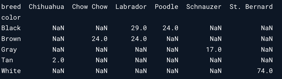
如果想要去除这些空值,可以设定参数 fill_value = 0 ,这样就用0替代了。
另外,如果设定 margin = True ,我们可以看到各类总的结果。(相当于多了一个行与列的sum)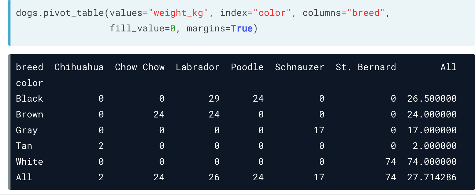
也可以利用切片及loc, iloc 对pivot_table进行处理。
如果想要计算其统计数据,可以直接调用 dataframe_pivot_table.mean() 。一般来说都有参数 axis , 默认为 index 或 row ,表示根据行或索引来划分计算。如果想要根据列,可以设定 axis = 'columns' 。
小彩蛋
用pandas 作图
pandas 也内置比较基本的作图工具。
比如 df['xx_col'].plot.hist() ,也可以做一个直方图。

若有收获,就点个赞吧
0 人点赞
