R 语言统计检验函数汇总

连续型数据

基于分布的检验

T检验

t.test(1:10, 10:20)

## 
##     Welch Two Sample t-test
## 
## data:  1:10 and 10:20
## t = -7, df = 19, p-value = 2e-06
## alternative hypothesis: true difference in means is not equal to 0
## 95 percent confidence interval:
##  -12.4  -6.6
## sample estimates:
## mean of x mean of y 
##       5.5      15.0

配对 t 检验：

t.test(rnorm(10), rnorm(10, mean = 1), paired = TRUE)

## 
##     Paired t-test
## 
## data:  rnorm(10) and rnorm(10, mean = 1)
## t = -2, df = 9, p-value = 0.03
## alternative hypothesis: true difference in means is not equal to 0
## 95 percent confidence interval:
##  -1.981 -0.096
## sample estimates:
## mean of the differences 
##                   -1.04

使用公式表示：

df <- data.frame(
  value = c(rnorm(10), rnorm(10, mean = 1)),
  group = c(rep("case", 10), rep("control", 10))
)
t.test(value ~ group, data = df)

## 
##     Welch Two Sample t-test
## 
## data:  value by group
## t = -0.7, df = 18, p-value = 0.5
## alternative hypothesis: true difference in means is not equal to 0
## 95 percent confidence interval:
##  -0.933  0.447
## sample estimates:
##    mean in group case mean in group control 
##                 0.539                 0.782

假设方差同质化：

t.test(value ~ group, data = df, var.equal = TRUE)

## 
##     Two Sample t-test
## 
## data:  value by group
## t = -0.7, df = 18, p-value = 0.5
## alternative hypothesis: true difference in means is not equal to 0
## 95 percent confidence interval:
##  -0.933  0.447
## sample estimates:
##    mean in group case mean in group control 
##                 0.539                 0.782

总体方差比较

var.test(value ~ group, data = df)

## 
##     F test to compare two variances
## 
## data:  value by group
## F = 0.8, num df = 9, denom df = 9, p-value = 0.8
## alternative hypothesis: true ratio of variances is not equal to 1
## 95 percent confidence interval:
##  0.202 3.269
## sample estimates:
## ratio of variances 
##              0.812

bartlett.test(value ~ group, data = df)

## 
##     Bartlett test of homogeneity of variances
## 
## data:  value by group
## Bartlett's K-squared = 0.09, df = 1, p-value = 0.8

多个组间均值的比较

两组以上的比较要使用ANOVA

aov(wt ~ factor(cyl), data = mtcars)

## Call:
##    aov(formula = wt ~ factor(cyl), data = mtcars)
## 
## Terms:
##                 factor(cyl) Residuals
## Sum of Squares         18.2      11.5
## Deg. of Freedom           2        29
## 
## Residual standard error: 0.63
## Estimated effects may be unbalanced

## 查看详细的信息
model.tables(aov(wt ~ factor(cyl), data = mtcars))

## Tables of effects
## 
##  factor(cyl) 
##           4       6      8
##     -0.9315 -0.1001  0.782
## rep 11.0000  7.0000 14.000

ANOVA 分析假设各组样本数据的方差是相等的，如果知道（或怀疑）不相等，可以使用 oneway.test() 函数。

oneway.test(wt ~ cyl, data = mtcars)

## 
##     One-way analysis of means (not assuming equal variances)
## 
## data:  wt and cyl
## F = 20, num df = 2, denom df = 19, p-value = 2e-05

多组样本的配对 t 检验

pairwise.t.test(mtcars$wt, mtcars$cyl)

## 
##     Pairwise comparisons using t tests with pooled SD 
## 
## data:  mtcars$wt and mtcars$cyl 
## 
##   4     6   
## 6 0.01  -   
## 8 6e-07 0.01
## 
## P value adjustment method: holm

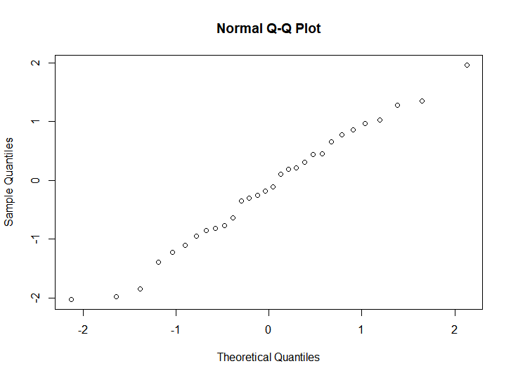
正态性检验

shapiro.test(rnorm(30))

## 
##     Shapiro-Wilk normality test
## 
## data:  rnorm(30)
## W = 1, p-value = 0.6

qqnorm(rnorm(30))

分布的对称性检验

用 Kolmogorov-Smirnov 检验查看一个向量是否来自一个对称的分布（不限于正态分布）。

ks.test(rnorm(10), pnorm)

## 
##     One-sample Kolmogorov-Smirnov test
## 
## data:  rnorm(10)
## D = 0.3, p-value = 0.2
## alternative hypothesis: two-sided

函数第 1 个参数指定待检验的数据，第 2个参数指定对称分布的类型，可以是数值型向量、指定概率分布函数的字符串或一个分布函数。

ks.test(rnorm(10), "pnorm")

## 
##     One-sample Kolmogorov-Smirnov test
## 
## data:  rnorm(10)
## D = 0.3, p-value = 0.3
## alternative hypothesis: two-sided

ks.test(rpois(10, lambda = 1), "pnorm")

## Warning in ks.test(rpois(10, lambda = 1), "pnorm"): ties should not be present for the
## Kolmogorov-Smirnov test

## 
##     One-sample Kolmogorov-Smirnov test
## 
## data:  rpois(10, lambda = 1)
## D = 0.5, p-value = 0.006
## alternative hypothesis: two-sided

检验两个向量是否服从同一分布

ks.test(rnorm(20), rnorm(30))

## 
##     Two-sample Kolmogorov-Smirnov test
## 
## data:  rnorm(20) and rnorm(30)
## D = 0.2, p-value = 0.4
## alternative hypothesis: two-sided

相关性分析

cor.test(mtcars$mpg, mtcars$wt)

## 
##     Pearson's product-moment correlation
## 
## data:  mtcars$mpg and mtcars$wt
## t = -10, df = 30, p-value = 1e-10
## alternative hypothesis: true correlation is not equal to 0
## 95 percent confidence interval:
##  -0.934 -0.744
## sample estimates:
##    cor 
## -0.868

不依赖分布的检验

均值检验

Wilcoxon 检验是 t 检验的非参数版本

## 秩和检验
wilcox.test(1:10, 10:20)

## Warning in wilcox.test.default(1:10, 10:20): cannot compute exact p-value with ties

## 
##     Wilcoxon rank sum test with continuity correction
## 
## data:  1:10 and 10:20
## W = 0.5, p-value = 1e-04
## alternative hypothesis: true location shift is not equal to 0

## 符号秩检验
wilcox.test(1:10, 10:19, paired = TRUE)

## Warning in wilcox.test.default(1:10, 10:19, paired = TRUE): cannot compute exact p-value with
## ties

## 
##     Wilcoxon signed rank test with continuity correction
## 
## data:  1:10 and 10:19
## V = 0, p-value = 0.002
## alternative hypothesis: true location shift is not equal to 0

多均值比较

## Kruskal-Wallis 秩和检验
kruskal.test(wt ~ factor(cyl), data = mtcars)

## 
##     Kruskal-Wallis rank sum test
## 
## data:  wt by factor(cyl)
## Kruskal-Wallis chi-squared = 23, df = 2, p-value = 1e-05

方差检验

使用Fligner-Killeen（中位数）检验完成不同组别的方差比较

fligner.test(wt ~ cyl, data = mtcars)

## 
##     Fligner-Killeen test of homogeneity of variances
## 
## data:  wt by cyl
## Fligner-Killeen:med chi-squared = 0.5, df = 2, p-value = 0.8

离散数据

比例检验

使用 prop.test() 比较两组观测值发生的概率是否有差异。

heads <- rbinom(1, size = 100, prob = .5)
prop.test(heads, 100)

## 
##     1-sample proportions test with continuity correction
## 
## data:  heads out of 100, null probability 0.5
## X-squared = 2, df = 1, p-value = 0.1
## alternative hypothesis: true p is not equal to 0.5
## 95 percent confidence interval:
##  0.477 0.677
## sample estimates:
##    p 
## 0.58

prop.test(heads, 100, p = 0.3, correct = FALSE)

## 
##     1-sample proportions test without continuity correction
## 
## data:  heads out of 100, null probability 0.3
## X-squared = 37, df = 1, p-value = 1e-09
## alternative hypothesis: true p is not equal to 0.3
## 95 percent confidence interval:
##  0.482 0.672
## sample estimates:
##    p 
## 0.58

二项式检验

binom.test(c(682, 243), p = 3/4)

## 
##     Exact binomial test
## 
## data:  c(682, 243)
## number of successes = 682, number of trials = 925, p-value = 0.4
## alternative hypothesis: true probability of success is not equal to 0.75
## 95 percent confidence interval:
##  0.708 0.765
## sample estimates:
## probability of success 
##                  0.737

列联表

确定两个分类变量是否相关

Fisher精确检验

TeaTasting <-
matrix(c(3, 1, 1, 3),
       nrow = 2,
       dimnames = list(Guess = c("Milk", "Tea"),
                       Truth = c("Milk", "Tea")))
fisher.test(TeaTasting, alternative = "greater")

## 
##     Fisher's Exact Test for Count Data
## 
## data:  TeaTasting
## p-value = 0.2
## alternative hypothesis: true odds ratio is greater than 1
## 95 percent confidence interval:
##  0.314   Inf
## sample estimates:
## odds ratio 
##       6.41

当样本数比较多时，使用卡方检验代替

chisq.test(TeaTasting)

## Warning in chisq.test(TeaTasting): Chi-squared approximation may be incorrect

## 
##     Pearson's Chi-squared test with Yates' continuity correction
## 
## data:  TeaTasting
## X-squared = 0.5, df = 1, p-value = 0.5

对于三变量的混合影响，使用 Cochran-Mantel-Haenszel 检验。

Rabbits <-
array(c(0, 0, 6, 5,
        3, 0, 3, 6,
        6, 2, 0, 4,
        5, 6, 1, 0,
        2, 5, 0, 0),
      dim = c(2, 2, 5),
      dimnames = list(
          Delay = c("None", "1.5h"),
          Response = c("Cured", "Died"),
          Penicillin.Level = c("1/8", "1/4", "1/2", "1", "4")))
Rabbits

## , , Penicillin.Level = 1/8
## 
##       Response
## Delay  Cured Died
##   None     0    6
##   1.5h     0    5
## 
## , , Penicillin.Level = 1/4
## 
##       Response
## Delay  Cured Died
##   None     3    3
##   1.5h     0    6
## 
## , , Penicillin.Level = 1/2
## 
##       Response
## Delay  Cured Died
##   None     6    0
##   1.5h     2    4
## 
## , , Penicillin.Level = 1
## 
##       Response
## Delay  Cured Died
##   None     5    1
##   1.5h     6    0
## 
## , , Penicillin.Level = 4
## 
##       Response
## Delay  Cured Died
##   None     2    0
##   1.5h     5    0

mantelhaen.test(Rabbits)

## 
##     Mantel-Haenszel chi-squared test with continuity correction
## 
## data:  Rabbits
## Mantel-Haenszel X-squared = 4, df = 1, p-value = 0.05
## alternative hypothesis: true common odds ratio is not equal to 1
## 95 percent confidence interval:
##   1.03 47.73
## sample estimates:
## common odds ratio 
##                 7

列联表非参数检验

Friedman 秩和检验是一个非参数版本的双边 ANOVA 检验。

## Hollander & Wolfe (1973), p. 140ff.
## Comparison of three methods ("round out", "narrow angle", and
##  "wide angle") for rounding first base.  For each of 18 players
##  and the three method, the average time of two runs from a point on
##  the first base line 35ft from home plate to a point 15ft short of
##  second base is recorded.
RoundingTimes <-
matrix(c(5.40, 5.50, 5.55,
         5.85, 5.70, 5.75,
         5.20, 5.60, 5.50,
         5.55, 5.50, 5.40,
         5.90, 5.85, 5.70,
         5.45, 5.55, 5.60,
         5.40, 5.40, 5.35,
         5.45, 5.50, 5.35,
         5.25, 5.15, 5.00,
         5.85, 5.80, 5.70,
         5.25, 5.20, 5.10,
         5.65, 5.55, 5.45,
         5.60, 5.35, 5.45,
         5.05, 5.00, 4.95,
         5.50, 5.50, 5.40,
         5.45, 5.55, 5.50,
         5.55, 5.55, 5.35,
         5.45, 5.50, 5.55,
         5.50, 5.45, 5.25,
         5.65, 5.60, 5.40,
         5.70, 5.65, 5.55,
         6.30, 6.30, 6.25),
       nrow = 22,
       byrow = TRUE,
       dimnames = list(1 : 22,
                       c("Round Out", "Narrow Angle", "Wide Angle")))
friedman.test(RoundingTimes)

## 
##     Friedman rank sum test
## 
## data:  RoundingTimes
## Friedman chi-squared = 11, df = 2, p-value = 0.004