purrr
purrr包是Hadley Wickham大神编写的高级函数编程语言包,它提供了大量的类map函数,使用函数式编程的思想,致力于减少R中的循环操作
map族函数
单参数计算
map族函数输入的数据类型是向量,函数将向量中的每一个元素带入运算,返回的也是一个具有同样长度、同样变量名的向量,返回的向量类型由函数的后缀决定。
map() # 返回一个列表(list) map_lgl() # 返回一个逻辑型向量 map_int() # 返回一个整数型向量 map_dbl() # 返回双精度数值向量 map_chr() # 返回字符串向量 map_dfc() # 返回数据框(column bind) map_dfr() # 返回数据框(row bind)
多参数计算
purrr中的map族函数提供了较apply族函数更为友好的数据输入形式,便于进行多参数操作
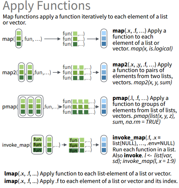
map() # Apply a function to each element (类似于apply的操作) map2() # Apply a function to pairs of elements (这个是2个输入参数的函数) pmap() # Apply a function to groups of elements (多参数形式) lmap() # Apply function to each list-element of a list or vector (类似于lapply) imap() # Apply .f to each element of a list or vector and its index. (对索引和内容同时操作) invoke_map() # Run each function in a list (每个元素使用不同的函数)
这些函数使用的示意图如下所示:
walk族函数
当我们使用函数的目的是向屏幕提供输出或将文件保存到磁盘——重要的是操作过程而不是返回值,我们应该使用游走函数,而不是map函数。
比如:
x = list(1, "a", 3)x %>%walk(print)#> [1] 1#> [1] "a"#> [1] 3
一般来说,walk()函数不如walk2()和pwalk()实用。例如有一个图形列表和一个文件名向量,那么我们就可以使用pwalk()将每个文件保存到相应的磁盘位置:
library(ggplot2)plots = mtcars %>%split(.$cyl) %>%map(~ggplot(., aes(mpg, wt)) + geom_point())paths = stringr::str_c(names(plots), ".pdf")pwalk(list(paths, plots), ggsave, path = tempdir())#> Saving 7 x 5 in image#> Saving 7 x 5 in image#> Saving 7 x 5 in image
list的处理操作
FILTER LISTS
pluck和chuck
pluck和chuck可以代替繁琐的[[]]操作,使list元素的选取更加简洁
> obj1 <- list("a", list(1, elt = "foo"))> obj2 <- list("b", list(2, elt = "bar"))> x <- list(obj1, obj2)> x[[1]][[1]][[1]][1] "a"[[1]][[2]][[1]][[2]][[1]][1] 1[[1]][[2]]$elt[1] "foo"[[2]][[2]][[1]][1] "b"[[2]][[2]][[2]][[2]][[1]][1] 2[[2]][[2]]$elt[1] "bar"> pluck(x, 1)[[1]][1] "a"[[2]][[2]][[1]][1] 1[[2]]$elt[1] "foo"> pluck(x, 1, 2)[[1]][1] 1$elt[1] "foo"> pluck(x, 1, 2, "elt")[1] "foo"> chuck(x, 1)[[1]][1] "a"[[2]][[2]][[1]][1] 1[[2]]$elt[1] "foo"> chuck(x, 1)[[1]][1] "a"[[2]][[2]][[1]][1] 1[[2]]$elt[1] "foo"
pluck和chuck的区别:当选取的元素不存在时,pluck返回NULL,而chuck会报错
条件选取
keep函数选取符合某一条件的元素discard函数相反,选取不符合某一条件的元素compact函数则去掉所有为空的元素
> x <- list(1,2,3) %>% keep(function(x)(x>2))> x[[1]][1] 3> x <- list(1,2,3) %>% discard(function(x)(x>2))> x[[1]][1] 1[[2]][1] 2> x <- list(1,2,3,NULL) %>% compact()> x[[1]][1] 1[[2]][1] 2[[3]][1] 3
head_while和tail_while
> pos <- function(x) x >= 0> head_while(5:-5, pos)[1] 5 4 3 2 1 0> pos <- function(x) x < 0> tail_while(5:-5, pos)[1] -1 -2 -3 -4 -5
SUMMARISE LISTS
every和some
判断元素是否满足条件
> y <- list(0:10, 5.5)> y %>% every(is.numeric)[1] TRUE> y %>% every(is.integer)[1] FALSE> y %>% some(is.integer)[1] TRUE
has_element
判断是否包含某一对象
> x <- list(1:10, 5, 9.9)> x %>% has_element(1:10)[1] TRUE> x %>% has_element(3)[1] FALSE
detect和detect_index
寻找匹配的第一个元素
> is_even <- function(x) x %% 2 == 0> 3:10 %>% detect(is_even)[1] 4> 3:10 %>% detect_index(is_even)[1] 2
vec_depth
计算list的深度
> x <- list(+ list(),+ list(list()),+ list(list(list(1)))+ )> vec_depth(x)[1] 5> x %>% map_int(vec_depth)[1] 1 2 4
TRANSFORM LISTS
modify
modify同样也是对列表或者向量中的元素进行函数运算,但是与map家族函数相比存在一些区别:
map家族函数往往返回一个特定类型的对象(数值,逻辑) modify函数返回的对象与输入对象的类型相一致 也就是说,modify是“真正”的对输入对象进行计算操作
> iris %>%modify_if(is.factor, as.character) %>%str()'data.frame': 150 obs. of 5 variables:$ Sepal.Length: num 5.1 4.9 4.7 4.6 5 5.4 4.6 5 4.4 4.9 ...$ Sepal.Width : num 3.5 3 3.2 3.1 3.6 3.9 3.4 3.4 2.9 3.1 ...$ Petal.Length: num 1.4 1.4 1.3 1.5 1.4 1.7 1.4 1.5 1.4 1.5 ...$ Petal.Width : num 0.2 0.2 0.2 0.2 0.2 0.4 0.3 0.2 0.2 0.1 ...$ Species : chr "setosa" "setosa" "setosa" "setosa" ...
modify函数的变形与map家族函数的使用是类似的
RESHAPE LISTS
flatten
去除list的一层层级关系,相当于将list压缩扁平化,但是得到的对象的类型是稳定可预测的(可以自己设置结果的类型)
> x <- rerun(2, sample(3))> x[[1]][1] 2 1 3[[2]][1] 3 1 2> x %>% flatten()[[1]][1] 2[[2]][1] 1[[3]][1] 3[[4]][1] 3[[5]][1] 1[[6]][1] 2> x %>% flatten_int()[1] 2 1 3 3 1 2
transpose
置换列表的索引顺序,其实就是将二级索引和一级索引的层级调换
> x <- rerun(3, x = runif(1), y = runif(3))> x[[1]][[1]]$x[1] 0.9489699[[1]]$y[1] 0.09894665 0.34629673 0.61291285[[2]][[2]]$x[1] 0.9344982[[2]]$y[1] 0.2195651 0.5119154 0.9527276[[3]][[3]]$x[1] 0.730148[[3]]$y[1] 0.3331638 0.9099907 0.4129223> transpose(x)$x$x[[1]][1] 0.9489699$x[[2]][1] 0.9344982$x[[3]][1] 0.730148$y$y[[1]][1] 0.09894665 0.34629673 0.61291285$y[[2]][1] 0.2195651 0.5119154 0.9527276$y[[3]][1] 0.3331638 0.9099907 0.4129223
JOIN (TO) LISTS
prepend
同append、splice函数共同实现list的合并
> x <- as.list(1:2)> x %>% append("a")[[1]][1] 1[[2]][1] 2[[3]][1] "a"> x %>% prepend("a")[[1]][1] "a"[[2]][1] 1[[3]][1] 2> x %>% prepend(list("a", "b"), before = 2)[[1]][1] 1[[2]][1] "a"[[3]][1] "b"[[4]][1] 2> splice(x, "a", "b")[[1]][1] 1[[2]][1] 2[[3]][1] "a"[[4]][1] "b"
WORK WITH LISTS
array_branch和array_tree
这两个函数的用法相同,会强制把数组转化成list
x <- array(1:12, c(2, 2, 3))> array_branch(x, 2)[[1]][,1] [,2] [,3][1,] 1 5 9[2,] 2 6 10[[2]][,1] [,2] [,3][1,] 3 7 11[2,] 4 8 12> array_branch(x, 3)[[1]][,1] [,2][1,] 1 3[2,] 2 4[[2]][,1] [,2][1,] 5 7[2,] 6 8[[3]][,1] [,2][1,] 9 11[2,] 10 12
总结
purrr包作为tidyverse的核心R包之一,提供了一些更加强大的编程工具,优化函数式编程的操作,对于数据分析的高效快速处理是十分重要的。

若有收获,就点个赞吧
0 人点赞
