什么是支撑向量机
svm 尝试寻找一个最优的决策边界
距离两个类别最近的样本最远
最近的样本称做支撑向量
SVM 最大化margin
线性可分 hard margin SVM
线性不可分 soft margin SVM
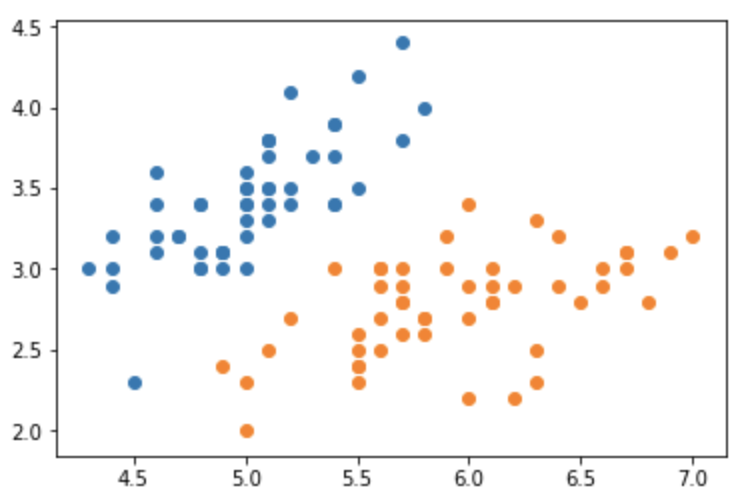
线性可分
from sklearn import datasetsimport numpy as npfrom matplotlib import pyplot as pltiris = datasets.load_iris()X = iris.datay = iris.targetX = X[y<2, :2]y = y[y<2]plt.scatter(X[y==0, 0], X[y==0, 1])plt.scatter(X[y==1, 0], X[y==1, 1])
from sklearn.preprocessing import StandardScalerstd = StandardScaler()X_STD = std.fit_transform(X)from sklearn.svm import LinearSVCsvc = LinearSVC(C=1e9)svc.fit(X_STD, y)def plot_decision_boundary(model, axis):x0, x1 = np.meshgrid(np.linspace(axis[0], axis[1], int((axis[1]-axis[0])*100)).reshape(-1, 1),np.linspace(axis[2], axis[3], int((axis[3]-axis[2])*100)).reshape(-1, 1),)X_new = np.c_[x0.ravel(), x1.ravel()]y_predict = model.predict(X_new)zz = y_predict.reshape(x0.shape)from matplotlib.colors import ListedColormapcustom_cmap = ListedColormap(['#EF9A9A','#FFF59D','#90CAF9'])plt.contourf(x0, x1, zz, linewidth=5, cmap=custom_cmap)plot_decision_boundary(svc, axis=[-3, 3, -3, 3])plt.scatter(X_STD[y==0, 0], X_STD[y==0, 1])plt.scatter(X_STD[y==1, 0], X_STD[y==1, 1])

svc2 = LinearSVC(C=0.01)svc2.fit(X_STD, y)plot_decision_boundary(svc2, axis=[-3, 3, -3, 3])plt.scatter(X_STD[y==0, 0], X_STD[y==0, 1])plt.scatter(X_STD[y==1, 0], X_STD[y==1, 1])

多项式特征
from sklearn import datasetsfrom sklearn.preprocessing import PolynomialFeaturesfrom sklearn.pipeline import PipelineX, y = datasets.make_moons(noise=0.15, random_state=666)plt.scatter(X[y==0, 0], X[y==0, 1])plt.scatter(X[y==1, 0], X[y==1, 1])

def PolynomialSVM(degree, C=1):return Pipeline([("poly", PolynomialFeatures(degree=degree)),("std", StandardScaler()),("svm", LinearSVC(C=C))])poly_svc = PolynomialSVM(3)poly_svc.fit(X, y)plot_decision_boundary(poly_svc, axis=[-1.5, 3, -1.5, 1.5])plt.scatter(X[y==0, 0], X[y==0, 1])plt.scatter(X[y==1, 0], X[y==1, 1])

多项式核
from sklearn.svm import SVCdef PolynomialKernelSVC(degree, C=1):return Pipeline([('std', StandardScaler()),('kernel_svc',SVC(kernel="poly", degree=degree, C=C))])poly_kernel_svc = PolynomialKernelSVC(5, 1)poly_kernel_svc.fit(X, y)plot_decision_boundary(poly_kernel_svc, axis=[-1.5, 3, -1.5, 1.5])plt.scatter(X[y==0, 0], X[y==0, 1])plt.scatter(X[y==1, 0], X[y==1, 1])

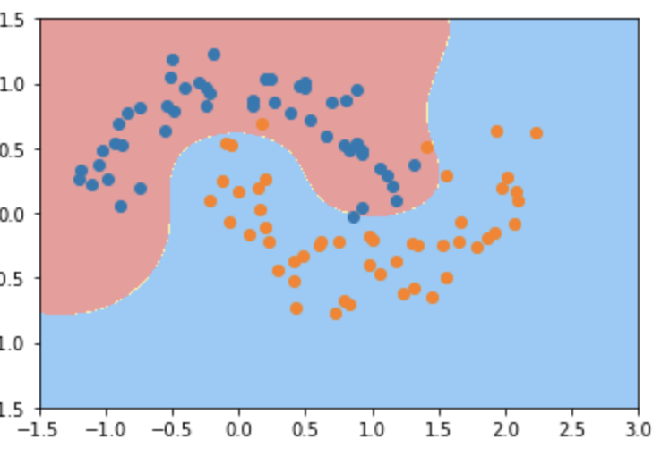
高斯核函数
def RBFKernelSVC(gamma=1):return Pipeline([('std', StandardScaler()),('svc', SVC(kernel='rbf', gamma=gamma))])rbf_svc = RBFKernelSVC()rbf_svc.fit(X, y)plot_decision_boundary(rbf_svc, axis=[-1.5, 3, -1.5, 1.5])plt.scatter(X[y==0, 0], X[y==0, 1])plt.scatter(X[y==1, 0], X[y==1, 1])
SVR线性模型
from sklearn.svm import SVRfrom sklearn.datasets import load_bostonX = load_boston().datay = load_boston().targetfrom sklearn.model_selection import train_test_splitX_train, X_test, y_train, y_test = train_test_split(X, y, random_state=666)def PolySVR(gamma):return Pipeline([('std', StandardScaler()),('svr', SVR(kernel='rbf', gamma=gamma))])poly_svr = PolySVR(0.1)poly_svr.fit(X_train, y_train)from sklearn.metrics import mean_squared_errormean_squared_error(y_test, poly_svr.predict(X_test))poly_svr.score(X_test, y_test)

若有收获,就点个赞吧
0 人点赞
