软件介绍
STREAM (Single-cell Trajectories Reconstruction, Exploration And Mapping) 软件是一个伪时间分析软件,通过一系列的特征选择,降纬(MLLE),轨迹推断(EPG)等步骤,逐步构建细胞发育轨迹,从而帮助我们更好的理解发育进化过程。
下载地址
github 地址:https://github.com/pinellolab/STREAM
安装本地版有两种方法,docker或者bioconda,我因为要安装在集群上,不具有管理员权限,所以,建议使用bioconda
conda 安装的方法就不说了,可以参考前文小白也看得懂的 ETE-toolkit 构建进化树流程
在终端配置 conda 的安装通道:
conda config --add channels defaultsconda config --add channels biocondaconda config --add channels conda-forge
创建一个stream的虚拟空间
conda create -n stream python=3.6 stream jupyterconda activate stream
使用命令行进行一键化分析
输入文件的格式
该流程需要输入三种文件(都是采用 tab 分割的 tsv 文件),分别是细胞表达矩阵,细胞注释名称以及细胞的颜色定义,当然,后面两个非必须,但是,还是提供比较好。
细胞表达矩阵示例:
| Name | AAACCTGGTATCAGTC-1_1 | AACCGCGCATTCCTGC-1_1 | AACGTTGAGCCCAATT-1_1 |
|---|---|---|---|
| GNLY | 0.142776811271601 | 0.181584363054937 | 0.152404882566299 |
| PAEP | 0.28157594020077 | 0.26124097727991 | 0.33343093647266 |
| MT1G | -0.0174682667681339 | 1.30917646946733 | 0.193603016988391 |
| HBB | …… | …… | …… |
| CD74 | …… | …… | …… |
表达矩阵可以是原始的 counts 值,也可以是经过标准化后的数据
细胞列表示例:
| MDSC |
| MDSC |
| Dendritic.cells.activated |
| MDSC |
| MDSC |
这里不需要输入标题栏,细胞名称和细胞 barcode 一一对应
颜色示例:
| DC2 | #66c2a5 |
| MDSC | #fc8d62 |
| Dendritic.cells.activated | #8da0cb |
你还可以选择一些有意识的基因出来做后续分析,这里不再展示。
可能很多人要问,如何从 Seurat 对象中获取该信息呢?翻一下官方文档可以知道:
library(Seurat)Seurat.obj<-readRDS("seurat.rds")#获取表达矩阵前,应该将默认矩阵转换为整合多样本的矩阵DefaultAssay(Seurat.obj) <- "integrated"expMat<-GetAssayData(Seurat.obj,slot="data")#data就是标准化后的数据,你也可以用countsexpMat<-as.data.frame(expMat)expMat$name<-rownames(expMat)expMat<-expMat[,c(ncols(expMat),1:(ncols(expMat)-1))]write.table(expMat,"data_Nestorowa.tsv",sep="\t",quote=FALSE,row.names=FALSE)#获取细胞信息就简单了cell<-as.data.frame(as.character(Idents(Seurat.obj)))write.table(cell,"cell_label.tsv",sep="\t",quote=FALSE,row.names=FALSE,col.names=FALSE)#映射颜色cell_c<-data.frame(cell=c("DC2","MDSC","Dendritic.cells.activated"),col=c("#66c2a5","#fc8d62","#8da0cb"))write.table(cell_c,"cell_label_color.tsv",sep="\t",quote=FALSE,col.names=FALSE)
命令行参数
-m, --matrixinput file name. Matrix is in .tsv or tsv.gz format in which each row represents a unique gene and each column is one cell. (default: None)-l, --cell_labelsfile name of cell labels (default: None)-c, --cell_labels_colorsfile name of cell label colors (default: None)-s, --select_featuresLOESS, PCA, all: Select variable genes using LOESS or top principal components using PCA or keep all the gene (default: LOESS)--TGdetect transition genes automatically--DEdetect DE genes automatically--LGetect leaf genes automatically-g, --gene_listgenes to visualize, it can either be filename which contains all the genes in one column or a set of gene names separated by comma (default: None)-p, --use_precomputeduse precomputed data files without re-computing structure learning part--log2perform log2 transformation--normnormalize data based on library size--atacindicate scATAC-seq data--n_processesSpecify the number of processes to use. (default, all the available cores).--loess_fracThe fraction of the data used in LOESS regression (default: 0.1)--pca_first_PCkeep first PC--pca_n_PCThe number of selected PCs (default: 15)--n_processesSpecify the number of processes to use. The default uses all the cores available--lle_neighboursLLE neighbour percent (default: 0.1)--lle_componentsNumber of components for LLE space (default: 3)--clusteringClustering method used for seeding the intial structure, choose from 'ap','kmeans','sc'.--dampingAffinity Propagation: damping factor (default: 0.75)--n_clustersNumber of clusters for spectral clustering or kmeans--EPG_n_nodesNumber of nodes for elastic principal graph (default: 50)--EPG_lambdalambda parameter used to compute the elastic energy (default: 0.02)--EPG_mumu parameter used to compute the elastic energy (default: 0.1)--EPG_trimmingradiusmaximal distance of point from a node to affect its embedment (default: Inf)--EPG_alphapositive numeric, alpha parameter of the penalized elastic energy (default: 0.02)--disable_EPG_optimizedisable optimizing branching--EPG_collapseCollapsing small branches--EPG_collapse_modethe mode used to collapse branches. It can be 'PointNumber','PointNumber_Extrema', 'PointNumber_Leaves','EdgesNumber' or 'EdgesLength' (default:'PointNumber')--EPG_collapse_parthe control parameter used for collapsing small branches--EPG_shiftshift branching point--EPG_shift_modethe mode to use to shift the branching points 'NodePoints' or 'NodeDensity' (default: NodeDensity)--EPG_shift_DRpositive numeric, the radius used when computing point density if EPG_shift_mode is 'NodeDensity' (default:0.05)--EPG_shift_maxshiftpositive integer, the maximum distance (number of edges) to consider when exploring the branching point neighborhood (default:5)--disable_EPG_extdisable extending leaves with additional nodes--EPG_ext_modethe mode used to extend the graph. It can be 'QuantDists', 'QuantCentroid' or 'WeigthedCentroid'. (default: QuantDists)--EPG_ext_parthe control parameter used for contribution of the different data points when extending leaves with nodes (default: 0.5)--DE_zscore_cutoffDifferentially Expressed Genes z-score cutoff (default: 2)--DE_logfc_cutoffDifferentially Expressed Genes log fold change cutoff (default: 0.25)--TG_spearman_cutoffTransition Genes Spearman correlation cutoff (default: 0.4)--TG_logfc_cutoffTransition Genes log fold change cutoff (default: 0.25)--LG_zscore_cutoffLeaf Genes z-score cutoff (default: 1.5)--LG_pvalue_cutoffLeaf Genes p value cutoff (default: 1e-2)--umapWhether to use UMAP for visualization (default: No)-rroot node for subwaymap_plot and stream_plot (default:None)--stream_log_viewuse log2 scale for y axis of stream_plot--for_webOutput files for website-o, --output_folderOutput folder (default: None)--newfile name of data to be mapped (default: None)--new_lfilename of new cell labels (default: None)--new_cfilename of new cell label colors (default: None)
使用默认参数运行:
stream -m data_Nestorowa.tsv -l cell_label.tsv -c cell_label_color.tsv
建议添加的参数:
stream -m data_Nestorowa.tsv -l cell_label.tsv -c cell_label_color.tsv --n_processes 4 --umap
这里因为使用的是标准化后的数据,所以跳过了标准化过程:否则添加--norm
进一步可视化基因:
stream -m data_Nestorowa.tsv -l cell_label.tsv -c cell_label_color.tsv -g gene_list.tsv -p
p参数可以避免重复计算,节省时间,默认会把所有节点都作为起始节点(根节点)计算一遍,你可以自己定义根节点-r
探索 Marker 基因:
stream -m data_Nestorowa.tsv -l cell_label.tsv -c cell_label_color.tsv --TG --DG --LG -p
结果
个人对于构建轨迹也不是太理解,就目前的理解来看,比较有用的结果是
- flat_tree.pdf
- subway_map.pdf
- std_vs_means.pdf
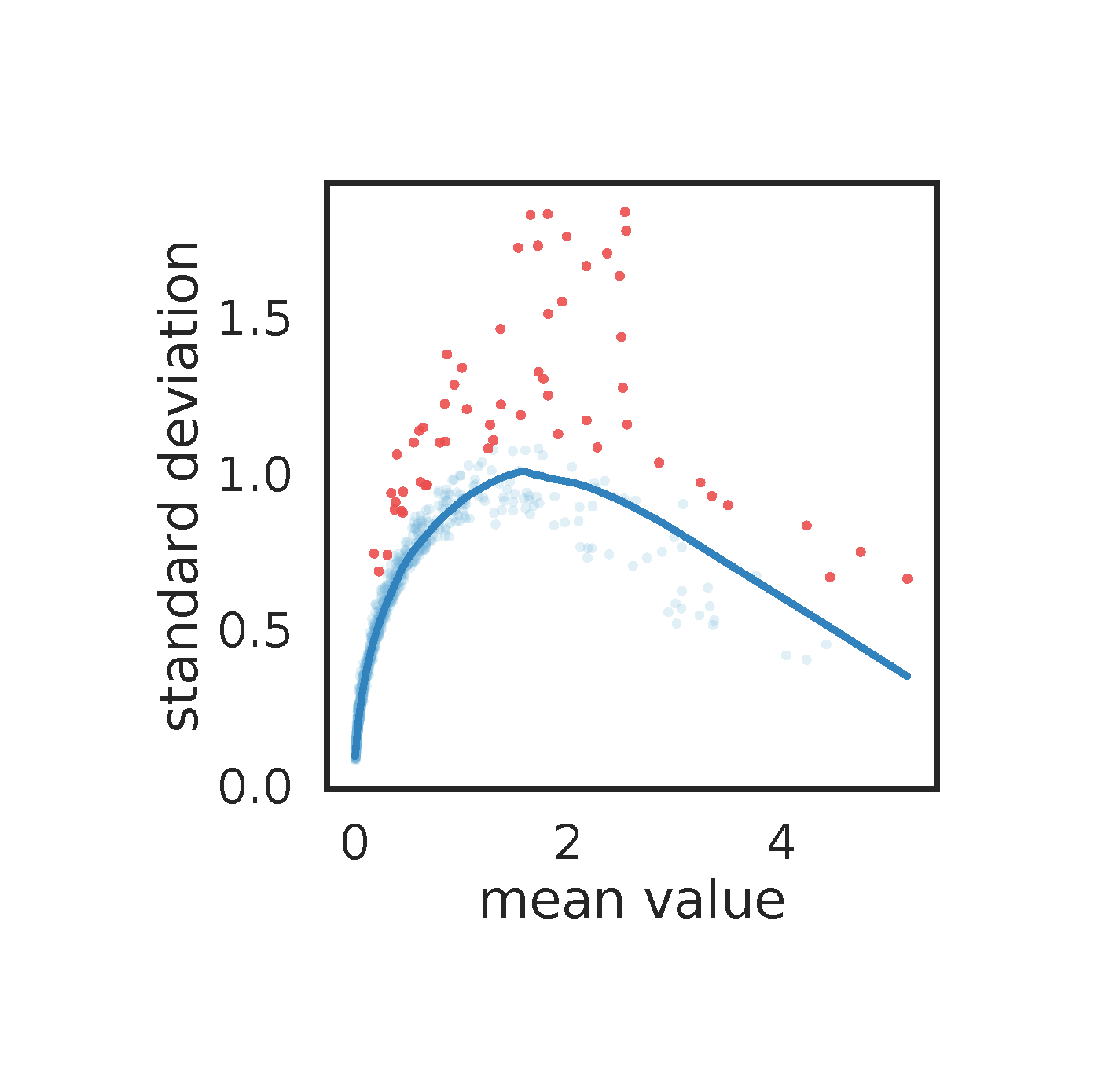
这个图是按照默认参数降纬跑的,这里需要注意的是,蓝线必须和点拟合的比较好才行,否则需要适当的调整参数
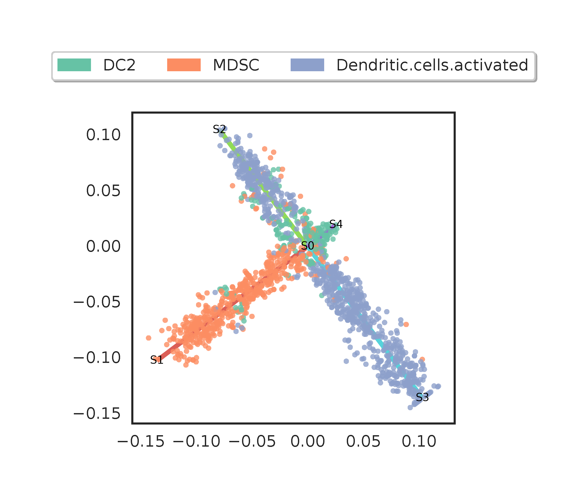
这张图应该是说,该细胞群由 S0 作为时间起点,向 S1,S2,S3 和 S4 分别进化出四支,就看我们选择哪一个作为根节点了。
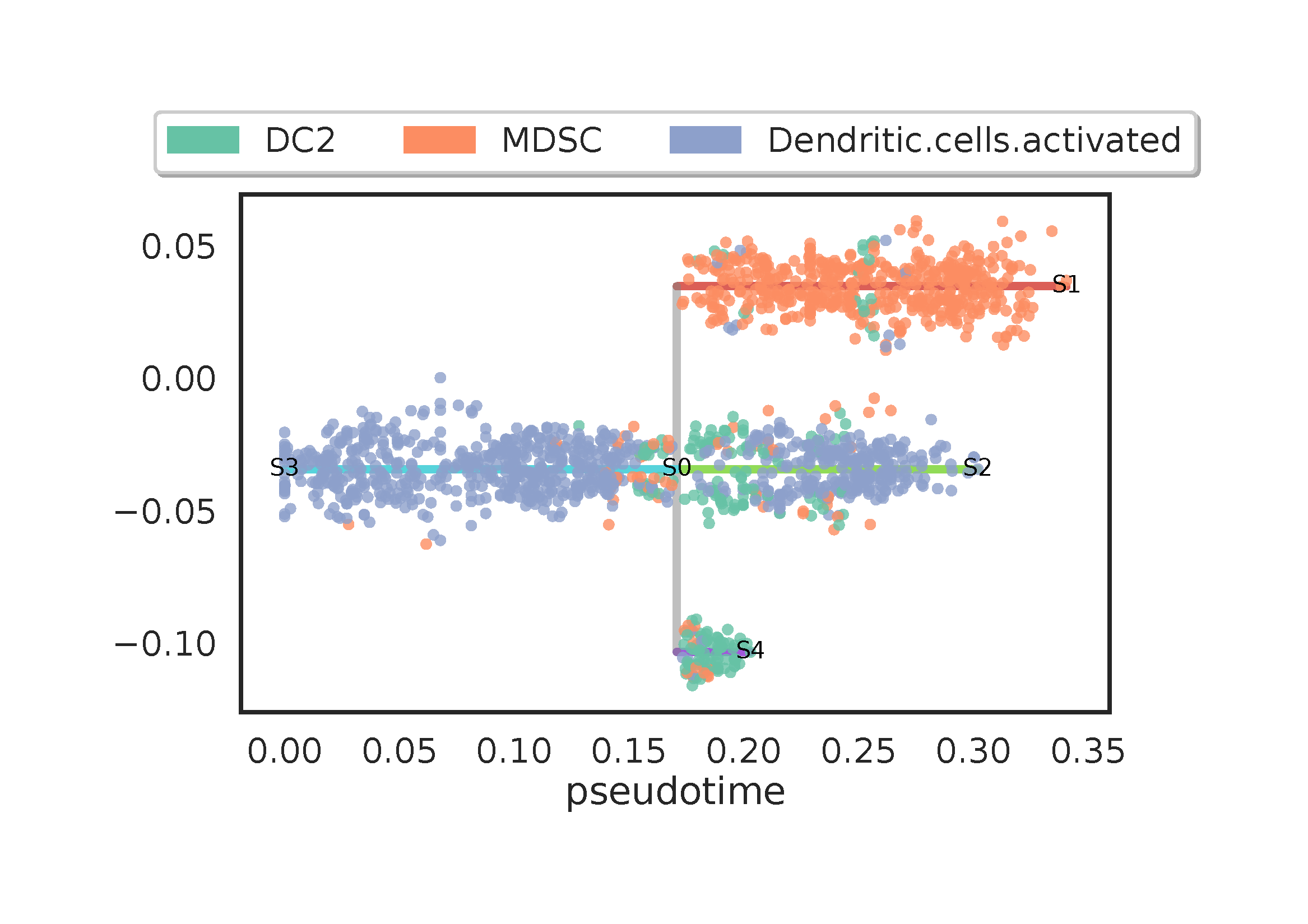
基于先验知识,激活的基因座细胞有可能作为发育的起点,所以我们选择 S3 作为根节点,构建出如上的时间序列。
以上,是采用一键化的方式计算,我们还可以使用交互的方式进行,但是因为我的集群没有可视化界面,操作起来就不方便,就没法演示了。具体方法可以参考
STREAM_scRNA-seq.ipynb
可视化网页版链接:http://stream.pinellolab.org

若有收获,就点个赞吧
0 人点赞
