import numpy as npimport pandas as pd
data = pd.read_csv(r"dataset/boston.csv", header=0)# data.drop(["class"], axis=1, inplace=True)data.head()
Unnamed: 0 crim zn indus chas nox rm age dis rad tax ptratio black lstat medv0 1 0.00632 18.0 2.31 0 0.538 6.575 65.2 4.0900 1 296 15.3 396.90 4.98 24.01 2 0.02731 0.0 7.07 0 0.469 6.421 78.9 4.9671 2 242 17.8 396.90 9.14 21.62 3 0.02729 0.0 7.07 0 0.469 7.185 61.1 4.9671 2 242 17.8 392.83 4.03 34.73 4 0.03237 0.0 2.18 0 0.458 6.998 45.8 6.0622 3 222 18.7 394.63 2.94 33.44 5 0.06905 0.0 2.18 0 0.458 7.147 54.2 6.0622 3 222 18.7 396.90 5.33 36.2
class LinearRegression:'''使用梯度下降回归算法'''def __init__(self, learning_rate, times):'''初始化parameters-----learn_rate: 学习率。梯度下降步长times: 迭代次数'''self.learning_rate = learning_rateself.times = timesdef fit(self, X, y):'''对样本进行预测Parameters:X: 特征矩阵,可以是List也可以是Ndarray,形状为: [样本数量,特征数量]y: 标签数组'''X = np.asarray(X)y = np.asarray(y)# 创建权重,初始值为0(也可以试试其他值),* 长度比X特征数多1,多出的就是w0self.w_ = np.zeros(1 + X.shape[1]) # X.shape[1] 为特征数# 创建损失值列表,用来每次迭代的损失值。# 损失值计算公式:(1/2 )*( 预测值 - 真实值)^2self.loss_ = []# 开始迭代for x in range(self.times):# 为什么使用 self.w_[1:] ? 因为X特征个数比w少1个,所以这里w0先去掉,点乘后再加上# 矩阵可以使用*运算,但是这里是ndarray数组只能用点乘,1表示x0y_hat = np.dot(X, self.w_[1:]) + self.w_[0]# 计算误差error = y - y_hat# 将损失值加入损失列表self.loss_.append(np.sum(error**2)/2)# 根据差距调整权重w_# 调整为 w(j)=w(j)+learn_rate*sum((y - y_hat)*x(j))# 更新w0,x看成1直接更新self.w_[0] += self.learning_rate * np.sum(error * 1)# ****************************************************# ************ 重点:这里一定要搞明白 ***************# ****************************************************# 使用x1到xn的某一列向量(即某一特征)的转置来更新w,也就是将w向x进拟合self.w_[1:] += self.learning_rate * np.dot(X.T, error)def predict(self, X):'''根据参数进行预测Paramaters-----X: [样本数量, 特征数量]-----Returns: 预测结果'''X = np.asarray(X)result = np.dot(X, self.w_[1:]) + self.w_[0]return result
class StandardScaler:'''对数据集进行标准化处理'''def fit(self, X):'''根据传递的样本,计算每个特征列的均值和标准差Parameters-----X: 训练数据。用来计算均值和标准差'''X = np.asarray(X)self.std_ = np.std(X, axis=0) # 按列计算标准差self.mean_ = np.mean(X, axis=0) # 按列计算#值def transform(self, X):'''对给定数据进行标准化处理* 将X每一列都变成标准正太分布的形式,即满足均值为0,标准差为1* 标准化也叫标准差标准化,经过处理的数据符合标准正态分布。Parameters-----X: 类数组类型。待转换的数据'''return (X - self.mean_) / self.std_def fit_transform(self, X):''' fit后transform'''self.fit(X)return self.transform(X)
lr = LinearRegression(learning_rate=0.001, times=20)t = data.sample(len(data), random_state=0)train_X = t.iloc[:400, :-1]train_y = t.iloc[:400, -1]test_X = t.iloc[400:, :-1]test_y = t.iloc[400:, -1]lr.fit(train_X, train_y)result = lr.predict(test_X)# display(result)display(np.mean((result - test_y)**2))display(lr.w_)display(lr.loss_)
1.1804176210461773e+210
array([-2.68833075e+099, -7.57608494e+101, -1.29174503e+100,
-2.67102000e+100, -3.24034515e+100, -1.81386180e+098,
-1.52555272e+099, -1.67597187e+100, -1.90402088e+101,
-9.69839266e+099, -3.06079801e+100, -1.19382162e+102,
-5.02206239e+100, -9.48116678e+101, -3.57226707e+100])
[116831.44,
2083552221174028.0,
4.883479637283036e+25,
1.14536821770387e+36,
2.686348040018552e+46,
6.300564127408661e+56,
1.477735116047291e+67,
3.465881830645266e+77,
8.128883677155966e+87,
1.9065494170189406e+98,
4.4716234404365476e+108,
1.0487751334726054e+119,
2.4597985390359684e+129,
5.769214638613026e+139,
1.353112339006075e+150,
3.1735914100271017e+160,
7.443345350908508e+170,
1.7457631703262697e+181,
4.09451517185836e+191,
9.603281119422997e+201]
# 为了避免每个特征数量级的不同对梯度下降造成的影响。我们对每个特征进行标准化lr = LinearRegression(learning_rate=0.0005, times=20)t = data.sample(len(data), random_state=0)train_X = t.iloc[:400, :-1]train_y = t.iloc[:400, -1]test_X = t.iloc[400:, :-1]test_y = t.iloc[400:, -1]# 标准化ss = StandardScaler()train_X = ss.fit_transform(train_X)test_X = ss.fit_transform(test_X)ss2 = StandardScaler()train_y = ss2.fit_transform(train_y)test_y = ss2.fit_transform(test_y)# 训练 预测lr.fit(train_X, train_y)result = lr.predict(test_X)display(np.mean((result - test_y)**2))display(lr.w_)display(lr.loss_)
0.14911890500740144
array([ 1.47715173e-16, -2.67726470e-03, -7.77999440e-02, 3.22218582e-02,
-4.15123849e-02, 7.21847299e-02, -1.22496354e-01, 3.18411097e-01,
-8.44203177e-03, -2.09306424e-01, 1.02744566e-01, -5.29297011e-02,
-1.81988334e-01, 9.71339528e-02, -3.93923586e-01])
[200.0, 109.56340745551384,
89.24537638439179,
79.69665810311717,
74.15994999919499,
70.76479029645887,
68.5986097420355,
67.15477786507567,
66.1444617646852,
65.4007703140392,
64.82595473196506,
64.36185638542904,
63.973228857262946,
63.638247945534275,
63.343061508525125,
63.07862649070146,
62.83885168788381,
62.619493019046615,
62.41748706751545,
62.23054285212329]
import matplotlib as mplimport matplotlib.pyplot as pltmpl.rcParams["font.family"] = "SimHei"mpl.rcParams["axes.unicode_minus"] = False
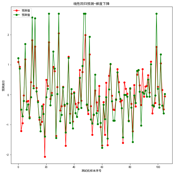
plt.figure(figsize=(10,10))plt.plot(result, "ro-", label="预测值")plt.plot(test_y.values, "go-", label="预测值") # pandas读取时serise类型,我们需要转为ndarrayplt.title("线性回归预测-梯度下降")plt.xlabel("测试机样本序号")plt.ylabel("预测房价")plt.legend()plt.show()
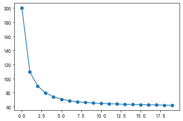
# 绘制累计误差值plt.plot(range(1,lr.times+1),lr.loss_, "o-")
# 因为放假更新涉及多个维度,不方便可视化# 为了可视化,我们只选择其中一个维度(RM),并画出直线,进行拟合lr = LinearRegression(learning_rate=0.0005, times=20)t = data.sample(len(data), random_state=0)train_X = t.iloc[:400, 6:7]train_y = t.iloc[:400, -1]test_X = t.iloc[400:, 5:6]test_y = t.iloc[400:, -1]# 标准化ss = StandardScaler()train_X = ss.fit_transform(train_X)test_X = ss.fit_transform(test_X)ss2 = StandardScaler()train_y = ss2.fit_transform(train_y)test_y = ss2.fit_transform(test_y)lr.fit(train_X, train_y)result = lr.predict(test_X)# display(result)display(np.mean((result - test_y)**2))
2.002805351917207
# 展示rm对对于价格的影响plt.scatter(train_X["rm"], train_y)# 展示权重display(lr.w_)# 构建方程 y = w0 + x*w1 = -3.05755421e-16 + x * 6.54993957e-01x = np.arange(-5,5,0.1)y = -3.05755421e-16 + x * 6.54993957e-01plt.plot(x, y, "g") # 绿色直线显示我们的拟合直线# ********* x.reshape(-1,1) 把一维转为二位 ****************plt.plot(x, lr.predict(x.reshape(-1,1)), 'r')# 可以看到我们预测的和你和的完全重合了
array([-3.05755421e-16, 6.54993957e-01])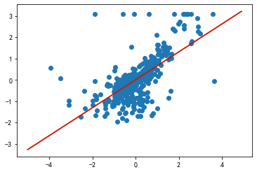

若有收获,就点个赞吧
0 人点赞
