7.1 模型量化技术
- 学习目标
- 相关知识
- 数据集说明
- 使用huggingface中的预训练BERT模型进行微调
  - 第一步: 安装核心的工具包并导入
用于设定全局配置的命名空间
from argparse import Namespace
从torch.utils.data中导入常用的模型处理工具，会在代码使用中进行详细介绍
from torch.utils.data import (DataLoader, RandomSampler, SequentialSampler,
TensorDataset)
模型进度可视化工具，在评估过程中，帮助打印进度条
from tqdm import tqdm
从transformers中导入BERT模型的相关工具
from transformers import (BertConfig, BertForSequenceClassification, BertTokenizer,)
从transformers中导入GLUE数据集的评估指标计算方法
from transformers import glue_compute_metrics as compute_metrics
从transformers中导入GLUE数据集的输出模式(回归/分类)
from transformers import glue_output_modes as output_modes
从transformers中导入GLUE数据集的预处理器processors
# processors是将持久化文件加载到内存的过程，即输入一般为文件路径，输出是训练数据和对应标签的某种数据结构，如列表表示。
from transformers import glue_processors as processors
从transformers中导入GLUE数据集的特征处理器convert_examples_to_features
# convert_examples_to_features是将processor的输出处理成模型需要的输入，NLP定中的一般流程为数值映射，指定长度的截断补齐等
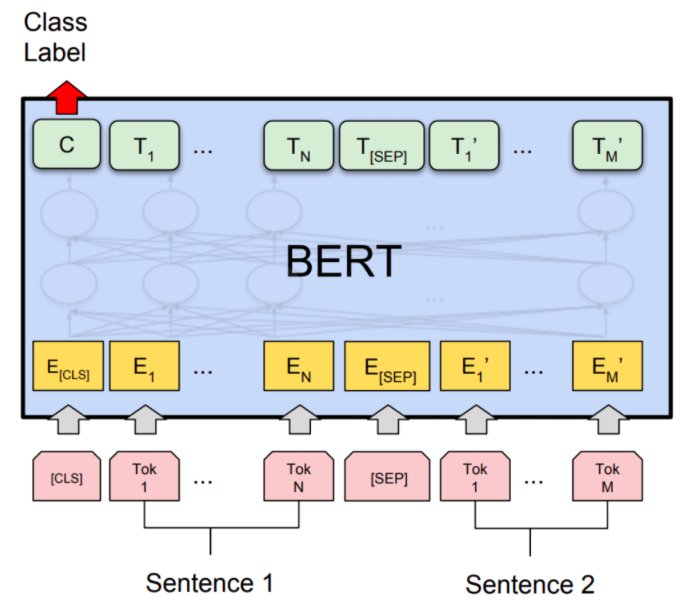
# 在BERT模型上处理句子对时，还需要在句子前插入[CLS]开始标记，在两个句子中间和第二个句子末端插入[SEP]分割/结束标记
from transformers import glue_convert_examples_to_features as convert_examples_to_features
设定与日志打印有关的配置
logger = logging.getLogger(name)
logging.basicConfig(format = ‘%(asctime)s - %(levelname)s - %(name)s - %(message)s’,
datefmt = ‘%m/%d/%Y %H:%M:%S’,
level = logging.WARN)
设置torch允许启动的线程数, 因为之后会对比压缩模型的耗时，因此防止该变量产生影响
torch.setnumthreads(1)
print(torch.__config.parallel_info())
- 第二步: 下载数据集并使用脚本进行微调
定义GLUE_DIR: 微调数据所在路径, 这里我们使用glue_data中的数据作为微调数据
export GLUE_DIR=./glue_data
# 定义OUT_DIR: 模型的保存路径, 我们将模型保存在当前目录的bert_finetuning_test文件中
export OUT_DIR=./bert_finetuning_test/
使用python运行微调脚本
# —model_type: 选择需要微调的模型类型, 这里可以选择BERT, XLNET, XLM, roBERTa, distilBERT, ALBERT
# —model_name_or_path: 选择具体的模型或者变体, 这里是在英文语料上微调, 因此选择bert-base-uncased
# —task_name: 它将代表对应的任务类型, 如MRPC代表句子对二分类任务
# —do_train: 使用微调脚本进行训练
# —do_eval: 使用微调脚本进行验证
# —data_dir: 训练集及其验证集所在路径, 将自动寻找该路径下的train.tsv和dev.tsv作为训练集和验证集
# —max_seq_length: 输入句子的最大长度, 超过则截断, 不足则补齐
# —learning_rate: 学习率
# —num_train_epochs: 训练轮数
# —output_dir $OUT_DIR: 训练后的模型保存路径
- 第三步: 设定全局配置并加载微调模型
实例化一个配置的命名空间
configs = Namespace()
模型的输出文件路径
configs.output_dir = “./bert_finetuning_test/“
验证数据集所在路径(与训练集相同)
configs.data_dir = “./glue_data/MRPC”
预训练模型的名字
configs.model_name_or_path = “bert-base-uncased”
文本的最大对齐长度
configs.max_seq_length = 128
GLUE中的任务名(需要小写)
configs.task_name = “MRPC”.lower()
根据任务名从GLUE数据集处理工具包中取出对应的预处理工具
configs.processor = processors configs.task_name
得到对应模型输出模式(MRPC为分类)
configs.output_mode = output_modes[configs.task_name]
得到该任务的对应的标签种类列表
configs.label_list = configs.processor.get_labels()
定义模型类型
configs.model_type = “bert”.lower()
是否全部使用小写文本
configs.do_lower_case = True
使用的设备
configs.device = “cpu”
# 每次验证的批次大小
configs.per_eval_batch_size = 8
gpu的数量
configs.n_gpu = 0
是否需要重写数据缓存
configs.overwrite_cache = False
- 加载微调模型
加载BERT预训练模型的数值映射器
tokenizer = BertTokenizer.from_pretrained(
configs.output_dir, do_lower_case=configs.do_lower_case)
加载带有文本分类头的BERT模型
model = BertForSequenceClassification.from_pretrained(configs.output_dir)
将模型传到制定设备上
model.to(configs.device)
- 第四步: 编写用于模型使用的评估函数
使用动态量化技术对训练后的bert模型进行压缩
- 第一步: 将模型应用动态量化技术
打印动态量化后的BERT模型
print(quantized_model)
- 第二步: 对比压缩后模型的大小
分别打印model和quantized_model
print_size_of_model(model)
print_size_of_model(quantized_model)
- 第三步: 对比压缩后的模型的推理准确性和耗时
- 第四步: 序列化模型以便之后使用
附录
- run_glue.py微调脚本代码
7.2 模型剪枝技术
- 学习目标
- 剪枝技术介绍与原理
- 使用prune对已有模型进行剪枝
  - 第一步：导入工具包并获得模型
这里不再对LeNet网络做过多的介绍，因为我们的重点是剪枝技术
# 无论你使用哪一种网络进行剪枝，你必须熟知这个网络中的组成部分即哪些能够剪枝
# 比如在这里，conv1，conv2，fc1，fc2，fc3都是可以被剪枝的
class LeNet(nn.Module):
def init(self):
super(LeNet, self).init()
self.conv1 = nn.Conv2d(1, 6, 3)
self.conv2 = nn.Conv2d(6, 16, 3)
self.fc1 = nn.Linear(16 5 5, 120) # 5x5 image dimension
self.fc2 = nn.Linear(120, 84)
self.fc3 = nn.Linear(84, 10)
获得这个模型对象
model = LeNet().to(device=device)
- 第二步：使用剪枝工具并了解其作用方式
- 第三步：持久化修剪后的模型
- 第四步：工程中常用的修剪方法
用元组指定需要剪枝的层和参数类型
parameters_to_prune = (
(model.conv1, ‘weight’),
(model.conv2, ‘weight’),
(model.fc1, ‘weight’),
(model.fc2, ‘weight’),
(model.fc3, ‘weight’),
)
进行全局剪枝，参数分别是需要剪枝的层和参数类型，剪枝方法，剪枝比例
# 通过这样的操作我们就可以得到剪枝后的模型，这里的0.2是整体的20%，各个部分剪枝在20%左右
# 这里使用了L1剪枝
prune.global_unstructured(
parameters_to_prune,
pruning_method=prune.L1Unstructured,
amount=0.2,
)
永久化参数
for module, name in parameters_to_prune:
prune.remove(module, name)
- #
小节总结
7.3 使用ONNX-Runtime进行模型推断加速
- 学习目标
- 什么是ONNX和ONNX-Runtime
- 使用ONNX-Runtime进行模型推断加速的步骤
  - 第一步：安装必备的工具包
  - 第二步：将已有模型转换成ONNX格式
这里以resnet18模型为例
model = torchvision.models.resnet18(pretrained=True)
# 随机初始化一个指定shape的输入
input = torch.randn(1, 3, 224, 224, requires_grad=True)
# 评估模式
model.eval()
使用torch.onnx导出resnet18.onnx
torch.onnx.export(model, input, onnx_model_name, input_names=input_names, output_names=output_names)
- 第三步：使用ONNX-Runtime进行模型预测
当前onnxruntime的输入要求的为numpy形式
def to_numpy(tensor):
“””将tensor转化成numpy”””
return tensor.detach().cpu().numpy() if tensor.requires_grad else tensor.cpu().numpy()
使用模型创建onnxruntime的session
ort_session = onnxruntime.InferenceSession(onnx_model_name)
# 在session中运行，要求输入为dict形式，key为之前定义好的input名字，且input必须为numpy形式
ort_outs = ort_session.run(None, {ort_session.get_inputs()[0].name: to_numpy(input)})
- 第四步：对比结果差异和推断时间
onnx模型的结果
ort_out = ort_outs[0]
对比两者在CPU上的预测时间差异
# 二者在GPU上的表现相当，因为onnxruntime本身也是调用cuda
onnx仅需8.5ms，大约节省2-3倍时间
0.008518030548095703
- ONNX-Runtime能够加速的原理
- 小节总结

7.1 模型量化技术

学习目标

了解模型压缩技术中的动态量化与静态量化的相关知识。
掌握使用huggingface中的预训练BERT模型进行微调。
掌握使用动态量化技术对训练后的bert模型进行压缩。

数据集说明

GLUE数据集合的介绍：
- GLUE由纽约大学，华盛顿大学，Google联合推出，涵盖不同的NLP任务类型，持续至2020年1月，其中包括11个子任务数据集，成为NLP研究发展的标准。我们这里使用其实MRPC数据集。
数据下载地址: 标准数据集一般使用下载脚本进行下载，会在之后的代码中演示。
MRPC数据集的任务类型：
- 句子对二分类任务
  - 训练集上正样本占68%，负样本占32%
- 评估指标这里使用：F1
- 评估指标计算方式：F1=2∗(precision∗recall)/(precision+recall)
数据集预览:
- MRPC数据集文件样式：

- MRPC/
- dev.tsv
- test.tsv
- train.tsv
- dev_ids.tsv
- msr_paraphrase_test.txt
- msr_paraphrase_train.txt

文件样式说明：

在使用中常用到的文件是train.tsv，dev.tsv，test.tsv，分别代表训练集，验证集和测试集。其中train.tsv与dev.tsv数据样式相同，都是带有标签的数据，其中test.tsv是不带有标签的数据。

train.tsv数据样式：

Quality #1 ID #2 ID #1 String #2 String
1 702876 702977 Amrozi accused his brother , whom he called “ the witness “ , of deliberately distorting his evidence . Referring to him as only “ the witness “ , Amrozi accused his brother of deliberately distorting his evidence .
0 2108705 2108831 Yucaipa owned Dominick ‘s before selling the chain to Safeway in 1998 for $ 2.5 billion . Yucaipa bought Dominick ‘s in 1995 for $ 693 million and sold it to Safeway for $ 1.8 billion in 1998 .
1 1330381 1330521 They had published an advertisement on the Internet on June 10 , offering the cargo for sale , he added . On June 10 , the ship ‘s owners had published an advertisement on the Internet , offering the explosives for sale .
0 3344667 3344648 Around 0335 GMT , Tab shares were up 19 cents , or 4.4 % , at A $ 4.56 , having earlier set a record high of A $ 4.57 . Tab shares jumped 20 cents , or 4.6 % , to set a record closing high at A $ 4.57 .
1 1236820 1236712 The stock rose $ 2.11 , or about 11 percent , to close Friday at $ 21.51 on the New York Stock Exchange . PG & E Corp. shares jumped $ 1.63 or 8 percent to $ 21.03 on the New York Stock Exchange on Friday .
1 738533 737951 Revenue in the first quarter of the year dropped 15 percent from the same period a year earlier . With the scandal hanging over Stewart ‘s company , revenue the first quarter of the year dropped 15 percent from the same period a year earlier .
0 264589 264502 The Nasdaq had a weekly gain of 17.27 , or 1.2 percent , closing at 1,520.15 on Friday . The tech-laced Nasdaq Composite .IXIC rallied 30.46 points , or 2.04 percent , to 1,520.15 .
1 579975 579810 The DVD-CCA then appealed to the state Supreme Court . The DVD CCA appealed that decision to the U.S. Supreme Court .
…

train.tsv数据样式说明：

train.tsv中的数据内容共分为5列，第一列数据，0或1，代表每对句子是否具有相同的含义，0代表含义不相同，1代表含义相同。第二列和第三列分别代表每对句子的id，第四列和第五列分别具有相同/不同含义的句子对。

test.tsv数据样式：

index #1 ID #2 ID #1 String #2 String
0 1089874 1089925 PCCW ‘s chief operating officer , Mike Butcher , and Alex Arena , the chief financial officer , will report directly to Mr So . Current Chief Operating Officer Mike Butcher and Group Chief Financial Officer Alex Arena will report to So .
1 3019446 3019327 The world ‘s two largest automakers said their U.S. sales declined more than predicted last month as a late summer sales frenzy caused more of an industry backlash than expected . Domestic sales at both GM and No. 2 Ford Motor Co. declined more than predicted as a late summer sales frenzy prompted a larger-than-expected industry backlash .
2 1945605 1945824 According to the federal Centers for Disease Control and Prevention ( news - web sites ) , there were 19 reported cases of measles in the United States in 2002 . The Centers for Disease Control and Prevention said there were 19 reported cases of measles in the United States in 2002 .
3 1430402 1430329 A tropical storm rapidly developed in the Gulf of Mexico Sunday and was expected to hit somewhere along the Texas or Louisiana coasts by Monday night . A tropical storm rapidly developed in the Gulf of Mexico on Sunday and could have hurricane-force winds when it hits land somewhere along the Louisiana coast Monday night .
4 3354381 3354396 The company didn ‘t detail the costs of the replacement and repairs . But company officials expect the costs of the replacement work to run into the millions of dollars .
5 1390995 1391183 The settling companies would also assign their possible claims against the underwriters to the investor plaintiffs , he added . Under the agreement , the settling companies will also assign their potential claims against the underwriters to the investors , he added .
6 2201401 2201285 Air Commodore Quaife said the Hornets remained on three-minute alert throughout the operation . Air Commodore John Quaife said the security operation was unprecedented .
7 2453843 2453998 A Washington County man may have the countys first human case of West Nile virus , the health department said Friday . The countys first and only human case of West Nile this year was confirmed by health officials on Sept . 8 .
…

test.tsv数据样式说明：

test.tsv中的数据内容共分为5列，第一列数据代表每条文本数据的索引；其余列的含义与train.tsv中相同。

使用huggingface中的预训练BERT模型进行微调

第一步: 安装必要的工具包并导入
第二步: 下载数据集并使用脚本进行微调
第三步: 设定全局配置并加载微调模型
第四步: 编写用于模型使用的评估函数

第一步: 安装核心的工具包并导入

安装核心工具包:

# 这是由huggingface提供的预训练模型使用工具包
pip install transformers==2.3.0

工具包导入

from __future__ import absolute_import, division, print_function

import logging
import numpy as np
import os
import random
import sys
import time
import torch

用于设定全局配置的命名空间
from argparse import Namespace

从torch.utils.data中导入常用的模型处理工具，会在代码使用中进行详细介绍
from torch.utils.data import (DataLoader, RandomSampler, SequentialSampler,
TensorDataset)

模型进度可视化工具，在评估过程中，帮助打印进度条
from tqdm import tqdm

从transformers中导入BERT模型的相关工具
from transformers import (BertConfig, BertForSequenceClassification, BertTokenizer,)

从transformers中导入GLUE数据集的评估指标计算方法
from transformers import glue_compute_metrics as compute_metrics

从transformers中导入GLUE数据集的输出模式(回归/分类)
from transformers import glue_output_modes as output_modes

从transformers中导入GLUE数据集的预处理器processors
# processors是将持久化文件加载到内存的过程，即输入一般为文件路径，输出是训练数据和对应标签的某种数据结构，如列表表示。
from transformers import glue_processors as processors

从transformers中导入GLUE数据集的特征处理器convert_examples_to_features
# convert_examples_to_features是将processor的输出处理成模型需要的输入，NLP定中的一般流程为数值映射，指定长度的截断补齐等
# 在BERT模型上处理句子对时，还需要在句子前插入[CLS]开始标记，在两个句子中间和第二个句子末端插入[SEP]分割/结束标记
from transformers import glue_convert_examples_to_features as convert_examples_to_features

设定与日志打印有关的配置
logger = logging.getLogger(name)
logging.basicConfig(format = ‘%(asctime)s - %(levelname)s - %(name)s - %(message)s’,
datefmt = ‘%m/%d/%Y %H:%M:%S’,
level = logging.WARN)

logging.getLogger(“transformers.modeling_utils”).setLevel(
logging.WARN) # Reduce logging

print(“torch version:”, torch.version)

设置torch允许启动的线程数, 因为之后会对比压缩模型的耗时，因此防止该变量产生影响
torch.setnumthreads(1)
print(torch.__config.parallel_info())

输出效果:

torch version: 1.3.1

ATen/Parallel:
at::get_num_threads() : 1
at::get_num_interop_threads() : 8
OpenMP 201511 (a.k.a. OpenMP 4.5)
omp_get_max_threads() : 1
Intel(R) Math Kernel Library Version 2019.0.4 Product Build 20190411 for Intel(R) 64 architecture applications
mkl_get_max_threads() : 1
Intel(R) MKL-DNN v0.20.5 (Git Hash 0125f28c61c1f822fd48570b4c1066f96fcb9b2e)
std::thread::hardware_concurrency() : 16
Environment variables:
OMP_NUM_THREADS : [not set]
MKL_NUM_THREADS : [not set]
ATen parallel backend: OpenMP

第二步: 下载数据集并使用脚本进行微调

下载GLUE中的MRPC数据集:

python download_glue_data.py --data_dir='./glue_data' --tasks='MRPC'

使用run_glue.py[具体代码内容见附录]进行模型微调:

# 注意: 这是一段使用shell运行的脚本, 运行过程中需要请求AWS的S3进行预训练模型下载

定义GLUE_DIR: 微调数据所在路径, 这里我们使用glue_data中的数据作为微调数据
export GLUE_DIR=./glue_data
# 定义OUT_DIR: 模型的保存路径, 我们将模型保存在当前目录的bert_finetuning_test文件中
export OUT_DIR=./bert_finetuning_test/

python ./run_glue.py \
—model_type bert \
—model_name_or_path bert-base-uncased \
—task_name MRPC \
—do_train \
—do_eval \
—do_lower_case \
—data_dir $GLUE_DIR/MRPC \
—max_seq_length 128 \
—per_gpu_eval_batch_size=8 \
—per_gpu_train_batch_size=8 \
—learning_rate 2e-5 \
—num_train_epochs 1.0 \
—output_dir $OUT_DIR

使用python运行微调脚本
# —model_type: 选择需要微调的模型类型, 这里可以选择BERT, XLNET, XLM, roBERTa, distilBERT, ALBERT
# —model_name_or_path: 选择具体的模型或者变体, 这里是在英文语料上微调, 因此选择bert-base-uncased
# —task_name: 它将代表对应的任务类型, 如MRPC代表句子对二分类任务
# —do_train: 使用微调脚本进行训练
# —do_eval: 使用微调脚本进行验证
# —data_dir: 训练集及其验证集所在路径, 将自动寻找该路径下的train.tsv和dev.tsv作为训练集和验证集
# —max_seq_length: 输入句子的最大长度, 超过则截断, 不足则补齐
# —learning_rate: 学习率
# —num_train_epochs: 训练轮数
# —output_dir $OUT_DIR: 训练后的模型保存路径

输出效果:

...
03/18/2020 00:55:17 - INFO - main - Loading features from cached file ./gluedata/MRPC/cachedtrainbert-base-uncased128mrpc
03/18/2020 00:55:17 - INFO - main - * Running training *
03/18/2020 00:55:17 - INFO - main - Num examples = 3668
03/18/2020 00:55:17 - INFO - main - Num Epochs = 1
03/18/2020 00:55:17 - INFO - main - Instantaneous batch size per GPU = 8
03/18/2020 00:55:17 - INFO - _main - Total train batch size (w. parallel, distributed & accumulation) = 8
03/18/2020 00:55:17 - INFO - __main - Gradient Accumulation steps = 1
03/18/2020 00:55:17 - INFO - __main - Total optimization steps = 459
Epoch: 0%| | 0/1 [00:00<?, ?it/s]
Iteration: 2%| | 8/459 [00:13<12:42, 1.69s/it]

运行成功后会在当前目录下生成 ./bert_finetuning_test文件夹，内部文件如下:

added_tokens.json checkpoint-200 checkpoint-350 eval_results.txt tokenizer_config.json
checkpoint-100 checkpoint-250 checkpoint-50 pytorch_model.bin training_args.bin
checkpoint-150 checkpoint-300 config.json special_tokens_map.json vocab.txt

第三步: 设定全局配置并加载微调模型

设定全局配置:

# 这些配置将在调用微调模型时进行使用

实例化一个配置的命名空间
configs = Namespace()

模型的输出文件路径
configs.output_dir = “./bert_finetuning_test/“

验证数据集所在路径(与训练集相同)
configs.data_dir = “./glue_data/MRPC”

预训练模型的名字
configs.model_name_or_path = “bert-base-uncased”

文本的最大对齐长度
configs.max_seq_length = 128

GLUE中的任务名(需要小写)
configs.task_name = “MRPC”.lower()

根据任务名从GLUE数据集处理工具包中取出对应的预处理工具
configs.processor = processorsconfigs.task_name

得到对应模型输出模式(MRPC为分类)
configs.output_mode = output_modes[configs.task_name]

得到该任务的对应的标签种类列表
configs.label_list = configs.processor.get_labels()

定义模型类型
configs.model_type = “bert”.lower()

是否全部使用小写文本
configs.do_lower_case = True

使用的设备
configs.device = “cpu”
# 每次验证的批次大小
configs.per_eval_batch_size = 8

gpu的数量
configs.n_gpu = 0

是否需要重写数据缓存
configs.overwrite_cache = False

加载微调模型:

# 因为在模型使用中，会使用一些随机方法，为了使每次运行的结果可以复现
# 需要设定确定的随机种子，保证每次随机化的数字在范围内浮动
def set_seed(seed):
random.seed(seed)
np.random.seed(seed)
torch.manual_seed(seed)
set_seed(42)

加载微调模型

加载BERT预训练模型的数值映射器
tokenizer = BertTokenizer.from_pretrained(
configs.output_dir, do_lower_case=configs.do_lower_case)

加载带有文本分类头的BERT模型
model = BertForSequenceClassification.from_pretrained(configs.output_dir)

将模型传到制定设备上
model.to(configs.device)

第四步: 编写用于模型使用的评估函数

def evaluate(args, model, tokenizer):
“””
模型评估函数
:param args: 模型的全局配置对象，里面包含模型的各种配置信息
:param model: 使用的模型
:param tokenizer: 文本数据的数值映射器
“””

# 因为之后会多次用到任务名和输出路径<br />    # 所以将其从参数中取出<br />    eval_task = args.task_name<br />    eval_output_dir = args.output_dir<br />    try:<br />        # 调用load_and_cache_examples加载原始或者已经缓存的数据<br />        # 得到一个验证数据集的迭代器对象<br />        eval_dataset = load_and_cache_examples(args, eval_task, tokenizer)
    # 判断模型输出路径是否存在<br />        if not os.path.exists(eval_output_dir):<br />            # 不存在的话，创建该路径<br />            os.makedirs(eval_output_dir)
    # 使用SequentialSampler封装验证数据集的迭代器对象<br />        # SequentialSampler是采样器对象，一般在Dataloader数据加载器中使用，<br />        # 因为数据加载器是以迭代的方式产生数据，因此每个批次数据可以指定采样规则，<br />        # SequentialSampler是顺序采样器，不改变原有数据集的顺序，依次取出数据。<br />        eval_sampler = SequentialSampler(eval_dataset)<br />        # 使用Dataloader数据加载器，参数分别是数据集的迭代器对象，采集器对象，批次大小<br />        eval_dataloader = DataLoader(eval_dataset, sampler=eval_sampler, batch_size=args.per_eval_batch_size)
    # 开始评估<br />        logger.info("***** Running evaluation *****")<br />        logger.info("  Num examples = %d", len(eval_dataset))<br />        logger.info("  Batch size = %d", args.per_eval_batch_size)<br />        # 初始化验证损失<br />        eval_loss = 0.0<br />        # 初始化验证步数<br />        nb_eval_steps = 0<br />        # 初始化预测的概率分布<br />        preds = None<br />        # 初始化输出真实标签值<br />        out_label_ids = None
    # 循环数据批次，使用tqdm封装数据加载器，可以在评估时显示进度条<br />        # desc是进度条前面的描述信息<br />        for batch in tqdm(eval_dataloader, desc="Evaluating"):<br />            # 评估过程中模型开启评估模式，不进行反向传播<br />            model.eval()<br />            # 从batch中取出数据的所有相关信息存于元组中<br />            batch = tuple(t.to(args.device) for t in batch)<br />            # 不进行梯度计算<br />            with torch.no_grad():<br />                # 将batch携带的数据信息表示称字典形式<br />                # 这些数据信息和load_and_cache_examples函数返回的数据对象中信息相同<br />                # 词汇的映射数值, 词汇的类型数值(0或1, 代表第一句和第二句话)<br />                # 注意力掩码张量，以及对应的标签<br />                inputs = {'input_ids':      batch[0],<br />                          'attention_mask': batch[1],<br />                          'token_type_ids': batch[2],<br />                          'labels':         batch[3]}<br />                # 将该字典作为参数输入到模型中获得输出<br />                outputs = model(**inputs)<br />                # 获得损失和预测分布<br />                tmp_eval_loss, logits = outputs<br />                # 将损失累加求均值<br />                eval_loss += tmp_eval_loss.mean().item()<br />            # 验证步数累加<br />            nb_eval_steps += 1
        # 如果是第一批次的数据<br />            if preds is None:<br />                # 结果分布就是模型的输出分布<br />                preds = logits.numpy()<br />                # 输出真实标签值为输入对应的labels<br />                out_label_ids = inputs['labels'].numpy()<br />            else:<br />                # 结果分布就是每一次模型输出分布组成的数组<br />                preds = np.append(preds, logits.numpy(), axis=0)<br />                # 输出真实标签值为每一次输入对应的labels组成的数组<br />                out_label_ids = np.append(out_label_ids, inputs['labels'].numpy(), axis=0)
    # 计算每一轮的平均损失<br />        eval_loss = eval_loss / nb_eval_steps<br />        # 取结果分布中最大的值对应的索引<br />        preds = np.argmax(preds, axis=1)<br />        # 使用compute_metrics计算对应的评估指标<br />        result = compute_metrics(eval_task, preds, out_label_ids)<br />        # 在日志中打印每一轮的评估结果<br />        logger.info("***** Eval results {} *****")<br />        logger.info(str(result))<br />    except Exception as e:<br />         print(e)<br />    return result

def loadand_cache_examples(args, task, tokenizer):
“””
加载或使用缓存数据
:param args: 全局配置参数
:param task: 任务名
:param tokenizer: 数值映射器
“””
# 根据任务名(MRPC)获得对应数据预处理器
processor = processorstask
# 获得输出模式
output_mode = output_modes[task]
# 定义缓存数据文件的名字
cached_features_file = os.path.join(args.data_dir, ‘cached{}{}{}_{}’.format(
‘dev’,
list(filter(None, args.model_name_or_path.split(‘/‘))).pop(),
str(args.max_seq_length),
str(task)))
# 判断缓存文件是否存在，以及全局配置中是否需要重写数据
if os.path.exists(cached_features_file) and not args.overwrite_cache:
# 使用torch.load(解序列化，一般用于加载模型，在这里用于加载训练数据)加载缓存文件
features = torch.load(cached_features_file)
else:
# 如果没有缓存文件，则需要使用processor从原始数据路径中加载数据
examples = processor.get_dev_examples(args.data_dir)
# 获取对应的标签
label_list = processor.get_labels()
# 再使用convert_examples_to_features生成模型需要的输入形式
features = convert_examples_to_features(examples,
tokenizer,
label_list=label_list,
max_length=args.max_seq_length,
output_mode=output_mode,
pad_token=tokenizer.convert_tokens_to_ids([tokenizer.pad_token])[0],
)
logger.info(“Saving features into cached file %s”, cached_features_file)
# 将其保存至缓存文件路径中
torch.save(features, cached_features_file)

# 为了有效利用内存，之后将使用数据加载器，我们需要在这里将张量数据转换成数据迭代器对象TensorDatase<br />    # TensorDataset：用于自定义训练数据结构的迭代封装器，它可以封装任何与训练数据映射值相关的数据<br />    #（如：训练数据对应的标签，训练数据使用的掩码张量，token的类型id等），<br />    # 它们必须能转换成张量，将同训练数据映射值一起在训练过程中迭代使用。
# 以下是分别把input_ids，attention_mask，token_type_ids，label封装在TensorDataset之中<br />    all_input_ids = torch.tensor([f.input_ids for f in features], dtype=torch.long)<br />    all_attention_mask = torch.tensor([f.attention_mask for f in features], dtype=torch.long)<br />    all_token_type_ids = torch.tensor([f.token_type_ids for f in features], dtype=torch.long)<br />    all_labels = torch.tensor([f.label for f in features], dtype=torch.long)<br />    dataset = TensorDataset(all_input_ids, all_attention_mask, all_token_type_ids, all_labels)<br />    # 返回数据迭代器对象<br />    return dataset

我们将在下面的模型量化中调用该评估函数。

使用动态量化技术对训练后的bert模型进行压缩

第一步: 将模型应用动态量化技术
第二步: 对比压缩后模型的大小
第三步: 对比压缩后的模型的推理准确性和耗时
第四步: 序列化模型以便之后使用

第一步: 将模型应用动态量化技术

应用动态量化技术:

# 使用torch.quantization.quantize_dynamic获得动态量化的模型
# 量化的网络层为所有的nn.Linear的权重，使其成为int8
quantized_model = torch.quantization.quantize_dynamic(
model, {torch.nn.Linear}, dtype=torch.qint8
)

打印动态量化后的BERT模型
print(quantized_model)

输出效果:

## 模型中的所有Linear层变成了DynamicQuantizedLinear层

BertForSequenceClassification(
(bert): BertModel(
(embeddings): BertEmbeddings(
(word_embeddings): Embedding(30522, 768, padding_idx=0)
(position_embeddings): Embedding(512, 768)
(token_type_embeddings): Embedding(2, 768)
(LayerNorm): LayerNorm((768,), eps=1e-12, elementwise_affine=True)
(dropout): Dropout(p=0.1, inplace=False)
)
(encoder): BertEncoder(
(layer): ModuleList(
(0): BertLayer(
(attention): BertAttention(
(self): BertSelfAttention(
(query): DynamicQuantizedLinear(in_features=768, out_features=768, scale=1.0, zero_point=0)
(key): DynamicQuantizedLinear(in_features=768, out_features=768, scale=1.0, zero_point=0)
(value): DynamicQuantizedLinear(in_features=768, out_features=768, scale=1.0, zero_point=0)
(dropout): Dropout(p=0.1, inplace=False)
)
(output): BertSelfOutput(
(dense): DynamicQuantizedLinear(in_features=768, out_features=768, scale=1.0, zero_point=0)
(LayerNorm): LayerNorm((768,), eps=1e-12, elementwise_affine=True)
(dropout): Dropout(p=0.1, inplace=False)
)
)
(intermediate): BertIntermediate(
(dense): DynamicQuantizedLinear(in_features=768, out_features=3072, scale=1.0, zero_point=0)
)
(output): BertOutput(
(dense): DynamicQuantizedLinear(in_features=3072, out_features=768, scale=1.0, zero_point=0)
(LayerNorm): LayerNorm((768,), eps=1e-12, elementwise_affine=True)
(dropout): Dropout(p=0.1, inplace=False)
)
)
(1): BertLayer(
(attention): BertAttention(
(self): BertSelfAttention(
(query): DynamicQuantizedLinear(in_features=768, out_features=768, scale=1.0, zero_point=0)
(key): DynamicQuantizedLinear(in_features=768, out_features=768, scale=1.0, zero_point=0)
(value): DynamicQuantizedLinear(in_features=768, out_features=768, scale=1.0, zero_point=0)
(dropout): Dropout(p=0.1, inplace=False)
)
(output): BertSelfOutput(
(dense): DynamicQuantizedLinear(in_features=768, out_features=768, scale=1.0, zero_point=0)
(LayerNorm): LayerNorm((768,), eps=1e-12, elementwise_affine=True)
(dropout): Dropout(p=0.1, inplace=False)
)
)
(intermediate): BertIntermediate(
(dense): DynamicQuantizedLinear(in_features=768, out_features=3072, scale=1.0, zero_point=0)
)
(output): BertOutput(
(dense): DynamicQuantizedLinear(in_features=3072, out_features=768, scale=1.0, zero_point=0)
(LayerNorm): LayerNorm((768,), eps=1e-12, elementwise_affine=True)
(dropout): Dropout(p=0.1, inplace=False)
)
)
…
…

    (11): BertLayer(<br />          (attention): BertAttention(<br />            (self): BertSelfAttention(<br />              (query): DynamicQuantizedLinear(in_features=768, out_features=768, scale=1.0, zero_point=0)<br />              (key): DynamicQuantizedLinear(in_features=768, out_features=768, scale=1.0, zero_point=0)<br />              (value): DynamicQuantizedLinear(in_features=768, out_features=768, scale=1.0, zero_point=0)<br />              (dropout): Dropout(p=0.1, inplace=False)<br />            )<br />            (output): BertSelfOutput(<br />              (dense): DynamicQuantizedLinear(in_features=768, out_features=768, scale=1.0, zero_point=0)<br />              (LayerNorm): LayerNorm((768,), eps=1e-12, elementwise_affine=True)<br />              (dropout): Dropout(p=0.1, inplace=False)<br />            )<br />          )<br />          (intermediate): BertIntermediate(<br />            (dense): DynamicQuantizedLinear(in_features=768, out_features=3072, scale=1.0, zero_point=0)<br />          )<br />          (output): BertOutput(<br />            (dense): DynamicQuantizedLinear(in_features=3072, out_features=768, scale=1.0, zero_point=0)<br />            (LayerNorm): LayerNorm((768,), eps=1e-12, elementwise_affine=True)<br />            (dropout): Dropout(p=0.1, inplace=False)<br />          )<br />        )<br />      )<br />    )<br />    (pooler): BertPooler(<br />      (dense): DynamicQuantizedLinear(in_features=768, out_features=768, scale=1.0, zero_point=0)<br />      (activation): Tanh()<br />    )<br />  )<br />  (dropout): Dropout(p=0.1, inplace=False)<br />  (classifier): DynamicQuantizedLinear(in_features=768, out_features=2, scale=1.0, zero_point=0)<br />)

第二步: 对比压缩后模型的大小

def print_size_of_model(model):
“””打印模型大小”””
# 保存模型中的参数部分到持久化文件
torch.save(model.state_dict(), “temp.p”)
# 打印持久化文件的大小
print(‘Size (MB):’, os.path.getsize(“temp.p”)/1e6)
# 移除该文件
os.remove(‘temp.p’)

分别打印model和quantized_model
print_size_of_model(model)
print_size_of_model(quantized_model)

输出效果:

## 模型参数文件大小缩减了257MB

Size (MB): 437.982584
Size (MB): 181.430351

第三步: 对比压缩后的模型的推理准确性和耗时

def time_model_evaluation(model, configs, tokenizer):
“””获得模型评估结果和运行时间”””
# 获得评估前时间
eval_start_time = time.time()
# 进行模型评估
result = evaluate(configs, model, tokenizer)
# 获得评估后时间
eval_end_time = time.time()
# 获得评估耗时
eval_duration_time = eval_end_time - eval_start_time
# 打印模型评估结果
print(“Evaluate result:”, result)
# 打印耗时
print(“Evaluate total time (seconds): {0:.1f}”.format(eval_duration_time))

输出效果:

Evaluating: 100%|██| 51/51 [01:36<00:00, 1.89s/it]
Evaluate result: {‘acc’: 0.8161764705882353, ‘f1’: 0.8739495798319329, ‘acc_and_f1’: 0.8450630252100841}
Evaluate total time (seconds): 96.4

Evaluating: 100%|███████████████████████████████| 51/51 [00:43<00:00, 1.19it/s]
Evaluate result: {‘acc’: 0.7965686274509803, ‘f1’: 0.8663446054750403, ‘acc_and_f1’: 0.8314566164630104}
Evaluate total time (seconds): 43.0

结论:
- 对模型进行动态量化后，参数文件大小明显减少。
- 动态量化后的模型在验证集上评估指标几乎不变，但是耗时却只用了原来的一半左右。

第四步: 序列化模型以便之后使用

# 量化模型的保存路径
quantized_output_dir = configs.output_dir + “quantized/“
# 判断是否需要创建该路径
if not os.path.exists(quantized_output_dir):
os.makedirs(quantized_output_dir)
# 使用save_pretrained保存模型
quantized_model.save_pretrained(quantized_output_dir)

输出效果:

# 在bert_finetuning_test/目录下

quantized/
- config.json
- pytorch_model.bin
附录
run_glue.py微调脚本代码
请访问: http://git.itcast.cn/Stephen/AI-key-file/blob/master/run_glue.py

7.2 模型剪枝技术

学习目标

了解模型剪枝原理。
掌握使用prune对已有模型进行剪枝。

剪枝技术介绍与原理

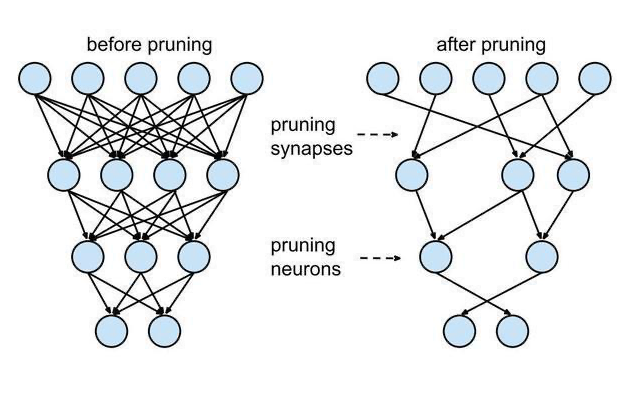
当前在NLP任务上取得优异成绩的模型往往是拥有大量参数的模型，如BERT，GPT等，但实际上，生物的高度文明是使用神经网络有效的稀疏连接，这正是“剪枝技术”的发展起源。而所谓剪枝技术原理，也就是将现有模型中的某些参数设置为0，等效于这些神经元失活。而参数置0的方式是使用MASK蒙版（蒙版0位置得到0，1位置得到原来的值）。下面我们将详细介绍这种技术的实现方式。

使用prune对已有模型进行剪枝

我们将使用torch.nn.utils.prune中的方法进行网络稀疏化，即剪枝。
要求torch版本应该>= 1.4.0。

pip install torch>=1.4.0

剪枝的讲解将分为以下步骤：
- 第一步：导入工具包并获得模型
- 第二步：使用剪枝工具并了解其作用方式
- 第三步：持久化修剪后的模型
- 第四步：工程中常用的修剪方法

第一步：导入工具包并获得模型

这里我们将使用LeNet作为剪枝的对象，当然你可以选择任何你已经训练好的某个网络和参数。

# 导入必备的工具包
import torch
from torch import nn
import torch.nn.utils.prune as prune
import torch.nn.functional as F

device = torch.device(“cuda” if torch.cuda.is_available() else “cpu”)

这里不再对LeNet网络做过多的介绍，因为我们的重点是剪枝技术
# 无论你使用哪一种网络进行剪枝，你必须熟知这个网络中的组成部分即哪些能够剪枝
# 比如在这里，conv1，conv2，fc1，fc2，fc3都是可以被剪枝的
class LeNet(nn.Module):
def init(self):
super(LeNet, self).init()
self.conv1 = nn.Conv2d(1, 6, 3)
self.conv2 = nn.Conv2d(6, 16, 3)
self.fc1 = nn.Linear(16 5 5, 120) # 5x5 image dimension
self.fc2 = nn.Linear(120, 84)
self.fc3 = nn.Linear(84, 10)

def forward(self, x):<br />        x = F.max_pool2d(F.relu(self.conv1(x)), (2, 2))<br />        x = F.max_pool2d(F.relu(self.conv2(x)), 2)<br />        x = x.view(-1, int(x.nelement() / x.shape[0]))<br />        x = F.relu(self.fc1(x))<br />        x = F.relu(self.fc2(x))<br />        x = self.fc3(x)<br />        return x

获得这个模型对象
model = LeNet().to(device=device)

第二步：使用剪枝工具并了解其作用方式

下面我们会使用剪枝工具并逐步查看参数的变化，先来看看没有剪枝之前的状态。

# 获得conv1模块
module = model.conv1
# 查看该模块的所有原生参数，一般由原生weight和原生bias组成
# 什么是原生参数呢？
# 这里是因为torch在设计存储网络参数时，允许为参数添加修改方式（如蒙版），
# 这些修改方式以buffer的形式存储，不会直接作用在named_parameters中的参数上，
# 因此把named_parameters中的参数叫做原生参数。
# 那如何获得作用了buffer之后的真实参数呢？
# 使用module.weight和module.bias即可
print(list(module.named_parameters()))

输出效果：

[('weight', Parameter containing:
tensor([[[[ 0.3161, -0.2212, 0.0417],
[ 0.2488, 0.2415, 0.2071],
[-0.2412, -0.2400, -0.2016]]],

    [[[ 0.0419,  0.3322, -0.2106],<br />          [ 0.1776, -0.1845, -0.3134],<br />          [-0.0708,  0.1921,  0.3095]]],
    [[[-0.2070,  0.0723,  0.2876],<br />          [ 0.2209,  0.2077,  0.2369],<br />          [ 0.2108,  0.0861, -0.2279]]],
    [[[-0.2799, -0.1527, -0.0388],<br />          [-0.2043,  0.1220,  0.1032],<br />          [-0.0755,  0.1281,  0.1077]]],
    [[[ 0.2035,  0.2245, -0.1129],<br />          [ 0.3257, -0.0385, -0.0115],<br />          [-0.3146, -0.2145, -0.1947]]],
    [[[-0.1426,  0.2370, -0.1089],<br />          [-0.2491,  0.1282,  0.1067],<br />          [ 0.2159, -0.1725,  0.0723]]]], device='cuda:0', requires_grad=True)),

(‘bias’, Parameter containing:
tensor([-0.1214, -0.0749, -0.2656, -0.1519, -0.1021, 0.1425], device=’cuda:0’,
requires_grad=True))]

# 查看参数修改方式即buffer
# 没有buffer的原生参数就是真实参数
print(list(module.named_buffers()))

输出效果：

[]

使用prune.random_unstructured随机方式进行剪枝

# 剪枝指定moudle即conv1中的weight参数，修剪（设置为0）30%
prune.random_unstructured(module, name=”weight”, amount=0.3)

# 查看修剪后的named_parameters参数
print(list(module.named_parameters()))

输出效果：

[('bias', Parameter containing:
tensor([-0.1214, -0.0749, -0.2656, -0.1519, -0.1021, 0.1425], device=’cuda:0’,
requires_grad=True)),

(‘weight_orig’, Parameter containing:
tensor([[[[ 0.3161, -0.2212, 0.0417],
[ 0.2488, 0.2415, 0.2071],
[-0.2412, -0.2400, -0.2016]]],

    [[[ 0.0419,  0.3322, -0.2106],<br />          [ 0.1776, -0.1845, -0.3134],<br />          [-0.0708,  0.1921,  0.3095]]],
    [[[-0.2070,  0.0723,  0.2876],<br />          [ 0.2209,  0.2077,  0.2369],<br />          [ 0.2108,  0.0861, -0.2279]]],
    [[[-0.2799, -0.1527, -0.0388],<br />          [-0.2043,  0.1220,  0.1032],<br />          [-0.0755,  0.1281,  0.1077]]],
    [[[ 0.2035,  0.2245, -0.1129],<br />          [ 0.3257, -0.0385, -0.0115],<br />          [-0.3146, -0.2145, -0.1947]]],
    [[[-0.1426,  0.2370, -0.1089],<br />          [-0.2491,  0.1282,  0.1067],<br />          [ 0.2159, -0.1725,  0.0723]]]], device='cuda:0', requires_grad=True))]

在结果中，我们发现原生参数并没有变化，而是名字由weight变成了weight_orig，进一步强调了它是原生参数。
为什么要进一步强调原生呢，是因为此时buffer中已经多了一些信息，原生参数和真实参数已经不再等价。

print(list(module.named_buffers()))

输出效果：

[('weight_mask', tensor([[[[0., 1., 0.],
[1., 0., 0.],
[1., 1., 1.]]],

    [[[1., 0., 1.],<br />          [1., 1., 0.],<br />          [1., 0., 1.]]],
    [[[1., 0., 0.],<br />          [0., 1., 1.],<br />          [1., 1., 1.]]],
    [[[1., 0., 0.],<br />          [1., 1., 1.],<br />          [1., 1., 1.]]],
    [[[1., 0., 1.],<br />          [1., 1., 1.],<br />          [0., 1., 1.]]],
    [[[1., 1., 1.],<br />          [1., 1., 0.],<br />          [1., 1., 0.]]]], device='cuda:0'))]

buffer中已经存在了用于剪枝的蒙版

使用module.weight查看真实使用参数：

print(module.weight)

输出效果：

tensor([[[[ 0.0000, -0.2212, 0.0000],
[ 0.2488, 0.0000, 0.0000],
[-0.2412, -0.2400, -0.2016]]],

    [[[ 0.0419,  0.0000, -0.2106],<br />          [ 0.1776, -0.1845, -0.0000],<br />          [-0.0708,  0.0000,  0.3095]]],
    [[[-0.2070,  0.0000,  0.0000],<br />          [ 0.0000,  0.2077,  0.2369],<br />          [ 0.2108,  0.0861, -0.2279]]],
    [[[-0.2799, -0.0000, -0.0000],<br />          [-0.2043,  0.1220,  0.1032],<br />          [-0.0755,  0.1281,  0.1077]]],
    [[[ 0.2035,  0.0000, -0.1129],<br />          [ 0.3257, -0.0385, -0.0115],<br />          [-0.0000, -0.2145, -0.1947]]],
    [[[-0.1426,  0.2370, -0.1089],<br />          [-0.2491,  0.1282,  0.0000],<br />          [ 0.2159, -0.1725,  0.0000]]]], device='cuda:0',<br />       grad_fn=<MulBackward0>)

第三步：持久化修剪后的模型

假如你已经对剪枝后的模型进行了必要的验证，并觉得它可以被保存并在将来部署使用，那么你需要持久化模型。

# 一般我们会首先将buffer中的蒙版永久作用在name_parameters中的参数上
# 这里的remove不是移除，而是永久化
prune.remove(module, ‘weight’)
print(list(module.named_parameters()))

输出效果：

[('bias_orig', Parameter containing:
tensor([-0.1214, -0.0749, -0.2656, -0.1519, -0.1021, 0.1425], device=’cuda:0’,
requires_grad=True)), (‘weight’, Parameter containing:
tensor([[[[ 0.0000, -0.2212, 0.0000],
[ 0.2488, 0.0000, 0.0000],
[-0.2412, -0.2400, -0.2016]]],

    [[[ 0.0000,  0.0000, -0.0000],<br />          [ 0.0000, -0.0000, -0.0000],<br />          [-0.0000,  0.0000,  0.0000]]],
    [[[-0.2070,  0.0000,  0.0000],<br />          [ 0.0000,  0.2077,  0.2369],<br />          [ 0.2108,  0.0861, -0.2279]]],
    [[[-0.0000, -0.0000, -0.0000],<br />          [-0.0000,  0.0000,  0.0000],<br />          [-0.0000,  0.0000,  0.0000]]],
    [[[ 0.2035,  0.0000, -0.1129],<br />          [ 0.3257, -0.0385, -0.0115],<br />          [-0.0000, -0.2145, -0.1947]]],
    [[[-0.0000,  0.0000, -0.0000],<br />          [-0.0000,  0.0000,  0.0000],<br />          [ 0.0000, -0.0000,  0.0000]]]], device='cuda:0', requires_grad=True))]

print(list(module.named_buffers()))

输出效果：

[]

此时buffer中已经没有任何修改，此时原生参数和真实参数等价。

保存序列化模型：

PATH = "./model.pth"
torch.save(model.state_dict(), PATH)
print(model.state_dict().keys())

输出效果：

odict_keys(['conv1.bias', 'conv1.weight', 'conv2.weight', 'conv2.bias', 'fc1.weight', 'fc1.bias', 'fc2.weight', 'fc2.bias', 'fc3.weight', 'fc3.bias'])

实际上假如你不进行prune.remove操作，直接保存state_dict()也是可以的，因为buffer也可以被保存在state_dict中，因为剪枝后往往需要继续重新训练，一般直到最后判断剪枝模型可用才使用remove永久化剪枝参数。

第四步：工程中常用的修剪方法

刚刚我们学习的都是“局部”的剪枝方式，而实际工程中我们往往直接针对模型进行整体剪枝。下面就是整体剪枝的方法：

# 获得模型
model = LeNet()

用元组指定需要剪枝的层和参数类型
parameters_to_prune = (
(model.conv1, ‘weight’),
(model.conv2, ‘weight’),
(model.fc1, ‘weight’),
(model.fc2, ‘weight’),
(model.fc3, ‘weight’),
)

进行全局剪枝，参数分别是需要剪枝的层和参数类型，剪枝方法，剪枝比例
# 通过这样的操作我们就可以得到剪枝后的模型，这里的0.2是整体的20%，各个部分剪枝在20%左右
# 这里使用了L1剪枝
prune.global_unstructured(
parameters_to_prune,
pruning_method=prune.L1Unstructured,
amount=0.2,
)

print(model.state_dict().keys())

print(“#################”)

永久化参数
for module, name in parameters_to_prune:
prune.remove(module, name)

print(model.state_dict().keys())

输出效果：

dict_keys(['conv1.bias', 'conv1.weight', 'conv2.weight', 'conv2.bias', 'fc1.weight', 'fc1.bias', 'fc2.weight', 'fc2.bias', 'fc3.weight', 'fc3.bias'])
odict_keys([‘conv1.bias’, ‘conv1.weight_orig’, ‘conv1.weight_mask’, ‘conv2.bias’, ‘conv2.weight_orig’, ‘conv2.weight_mask’, ‘fc1.bias’, ‘fc1.weight_orig’, ‘fc1.weight_mask’, ‘fc2.bias’, ‘fc2.weight_orig’, ‘fc2.weight_mask’, ‘fc3.bias’, ‘fc3.weight_orig’, ‘fc3.weight_mask’])

#

odict_keys([‘conv1.bias’, ‘conv1.weight’, ‘conv2.weight’, ‘conv2.bias’, ‘fc1.weight’, ‘fc1.bias’, ‘fc2.weight’, ‘fc2.bias’, ‘fc3.weight’, ‘fc3.bias’])
odict_keys([‘conv1.bias’, ‘conv1.weight’, ‘conv2.bias’, ‘conv2.weight’, ‘fc1.bias’, ‘fc1.weight’, ‘fc2.bias’, ‘fc2.weight’, ‘fc3.bias’, ‘fc3.weight’])

检查一下全局剪枝的20%在各个层中剪枝占比:

print(
“Sparsity in conv1.weight: {:.2f}%”.format(
100. float(torch.sum(model.conv1.weight == 0))
/ float(model.conv1.weight.nelement())
)
)
print(
“Sparsity in conv2.weight: {:.2f}%”.format(
100. float(torch.sum(model.conv2.weight == 0))
/ float(model.conv2.weight.nelement())
)
)
print(
“Sparsity in fc1.weight: {:.2f}%”.format(
100. float(torch.sum(model.fc1.weight == 0))
/ float(model.fc1.weight.nelement())
)
)
print(
“Sparsity in fc2.weight: {:.2f}%”.format(
100. float(torch.sum(model.fc2.weight == 0))
/ float(model.fc2.weight.nelement())
)
)
print(
“Sparsity in fc3.weight: {:.2f}%”.format(
100. float(torch.sum(model.fc3.weight == 0))
/ float(model.fc3.weight.nelement())
)
)
print(
“Global sparsity: {:.2f}%”.format(
100. float(
torch.sum(model.conv1.weight == 0)
+ torch.sum(model.conv2.weight == 0)
+ torch.sum(model.fc1.weight == 0)
+ torch.sum(model.fc2.weight == 0)
+ torch.sum(model.fc3.weight == 0)
)
/ float(
model.conv1.weight.nelement()
+ model.conv2.weight.nelement()
+ model.fc1.weight.nelement()
+ model.fc2.weight.nelement()
+ model.fc3.weight.nelement()
)
)
)

输出效果：

Sparsity in conv1.weight: 7.41%
Sparsity in conv2.weight: 9.49%
Sparsity in fc1.weight: 22.00%
Sparsity in fc2.weight: 12.28%
Sparsity in fc3.weight: 9.76%
Global sparsity: 20.00%

常用的剪枝方式解释：
- RandomUnstructured：随机剪枝
- L1Unstructured：按照L1范数（绝对值大小）剪枝，因为数值越小对结果的扰动也越小。

小节总结

学习了模型剪枝原理
学习了使用prune对已有模型进行剪枝
- 第一步：导入工具包并获得模型
- 第二步：使用剪枝工具并了解其作用方式
- 第三步：持久化修剪后的模型
- 第四步：工程中常用的修剪方法

7.3 使用ONNX-Runtime进行模型推断加速

学习目标

了解ONNX及其ONNX-Runtime的主要作用。
掌握如何使用ONNX-Runtime进行模型推断加速。

什么是ONNX和ONNX-Runtime

ONNX（Open Neural Network Exchange）开放式神经网络交换格式，与torch的pth，keras的h5，tensorflow的pb一样，它属于一种模型格式。
这种交换格式被设计的初衷：希望各种模型框架训练得到的模型能够通用。而现在它已经结合ONNX-Runtime成为一种加速模型推理的方法。
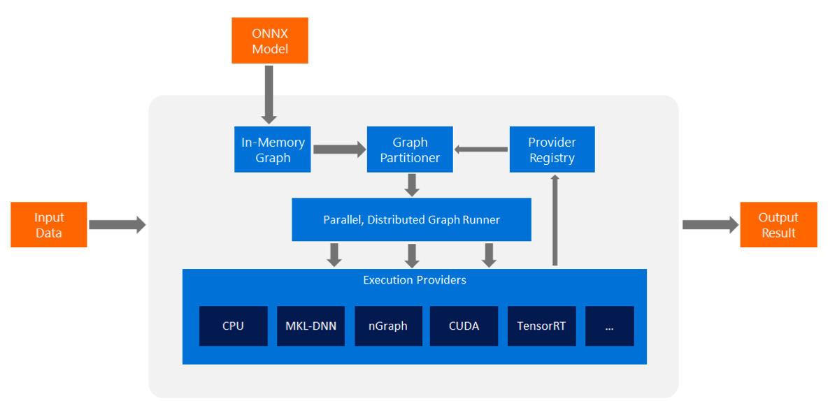
ONNX-Runtime就是指ONNX格式模型的运行环境，它由微软开源，该环境集成多种模型加速工具，如Nvidia的TensorRT等，用于快速模型推断。
能够原生支持ONNX模型转换的模型包括Pytorch，MXNET，Caffe2等框架（Tensorflow不可以）。

图中，蓝色的部分就是ONNX-Runtime，它能够自动利用已有设备上的各种加速工具，完成模型加速，无需人工参与，只需要我们将ONNX格式的模型作为输入即可。

使用ONNX-Runtime进行模型推断加速的步骤

第一步：安装必备的工具包
第二步：将已有模型转换成ONNX格式
第三步：使用ONNX-Runtime进行模型预测
第四步：对比结果差异和推断时间

第一步：安装必备的工具包

# onnx 1.7.0
# onnxruntime 1.4.0
pip install onnx onnxruntime

第二步：将已有模型转换成ONNX格式

import torch
import torch.onnx
import torchvision

这里以resnet18模型为例
model = torchvision.models.resnet18(pretrained=True)
# 随机初始化一个指定shape的输入
input = torch.randn(1, 3, 224, 224, requires_grad=True)
# 评估模式
model.eval()

# 定义onnx输入输出的名字（格式需要）
input_names = [“input1”]
output_names = [“output1”]

onnx_model_name = “resnet18.onnx”

使用torch.onnx导出resnet18.onnx
torch.onnx.export(model, input, onnx_model_name, input_names=input_names, output_names=output_names)

输出效果:

在该脚本路径下得到resnet18.onnx格式的模型。

第三步：使用ONNX-Runtime进行模型预测

import onnxruntime

当前onnxruntime的输入要求的为numpy形式
def to_numpy(tensor):
“””将tensor转化成numpy”””
return tensor.detach().cpu().numpy() if tensor.requires_grad else tensor.cpu().numpy()

使用模型创建onnxruntime的session
ort_session = onnxruntime.InferenceSession(onnx_model_name)
# 在session中运行，要求输入为dict形式，key为之前定义好的input名字，且input必须为numpy形式
ort_outs = ort_session.run(None, {ort_session.get_inputs()[0].name: to_numpy(input)})

第四步：对比结果差异和推断时间

# pth模型的结果
torch_out = to_numpy(model(input))

onnx模型的结果
ort_out = ort_outs[0]

print(torch_out)
print()
print(ort_out)

输出效果:

## 结果是一模一样的，没有任何差异

[[ 6.46063685e-01 2.58094740e+00 2.67934680e+00 2.84586716e+00
4.45001364e+00 3.60939002e+00 3.51634717e+00 2.71348268e-01
-1.15397012e+00 -7.00954318e-01 -7.89242506e-01 9.08504605e-01
1.55155942e-01 1.08485329e+00 1.31591737e+00 5.42257011e-01]]

import time

对比两者在CPU上的预测时间差异
# 二者在GPU上的表现相当，因为onnxruntime本身也是调用cuda

start = time.time()
torch_out = model(input)
end = time.time()
print(end - start)

start = time.time()
ort_outs = ort_session.run(None, {“input1”: to_numpy(input)})
end = time.time()
print(end - start)

输出效果:

# pth模型推断时间为24.6ms
0.024605449676513672

onnx仅需8.5ms，大约节省2-3倍时间
0.008518030548095703

ONNX-Runtime能够加速的原理

下面以其调用TensorRT(nvidia加速工具)加速BERT为例进行说明：

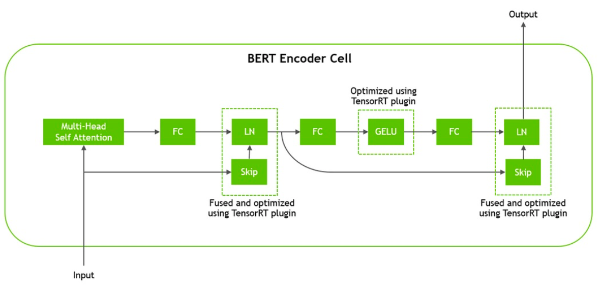
在BERT编码器中，将LayerNormalization层和残差连接进行融合以加速计算。
对gelu激活函数使用简化gelu计算方法加速计算。

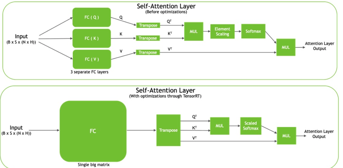
对所有的self-attention layer中的全连接层进行融合，以减少内存和正反向传播次数加速计算。
ONNX-Runtime内置针对主流模型（BERT，RESNET等）的并行计算模式，实现加速计算。

小节总结

学习了使用ONNX-Runtime进行模型推断加速的步骤：
- 第一步：安装必备的工具包
- 第二步：将已有模型转换成ONNX格式
- 第三步：使用ONNX-Runtime进行模型预测
- 第四步：对比结果差异和推断时间

ONNX-Runtime能够加速的原因：
- 1，作为加速工具的集成环境，能够自动调用加速工具cuda，TensorRT，nGragh等。
- 2，对特定模型的层和张量进行融合，以减少正反向传播次数。
- 3，对特定激活函数gelu进行简化计算。
- 4，针对主流模型（BERT，RESNET等）的并行计算模式，实现加速计算。

七、模型压缩与推断加速技术

7.1 模型量化技术

学习目标

相关知识

数据集说明

使用huggingface中的预训练BERT模型进行微调

第一步: 安装核心的工具包并导入

用于设定全局配置的命名空间from argparse import Namespace

从torch.utils.data中导入常用的模型处理工具，会在代码使用中进行详细介绍from torch.utils.data import (DataLoader, RandomSampler, SequentialSampler, TensorDataset)

模型进度可视化工具，在评估过程中，帮助打印进度条from tqdm import tqdm

从transformers中导入BERT模型的相关工具from transformers import (BertConfig, BertForSequenceClassification, BertTokenizer,)

从transformers中导入GLUE数据集的评估指标计算方法from transformers import glue_compute_metrics as compute_metrics

从transformers中导入GLUE数据集的输出模式(回归/分类)from transformers import glue_output_modes as output_modes

从transformers中导入GLUE数据集的预处理器processors# processors是将持久化文件加载到内存的过程，即输入一般为文件路径，输出是训练数据和对应标签的某种数据结构，如列表表示。from transformers import glue_processors as processors

设定与日志打印有关的配置logger = logging.getLogger(name)logging.basicConfig(format = ‘%(asctime)s - %(levelname)s - %(name)s - %(message)s’, datefmt = ‘%m/%d/%Y %H:%M:%S’, level = logging.WARN)

设置torch允许启动的线程数, 因为之后会对比压缩模型的耗时，因此防止该变量产生影响torch.setnumthreads(1)print(torch.__config.parallel_info())

第二步: 下载数据集并使用脚本进行微调

定义GLUE_DIR: 微调数据所在路径, 这里我们使用glue_data中的数据作为微调数据export GLUE_DIR=./glue_data# 定义OUT_DIR: 模型的保存路径, 我们将模型保存在当前目录的bert_finetuning_test文件中export OUT_DIR=./bert_finetuning_test/

第三步: 设定全局配置并加载微调模型

实例化一个配置的命名空间configs = Namespace()

模型的输出文件路径configs.output_dir = “./bert_finetuning_test/“

验证数据集所在路径(与训练集相同)configs.data_dir = “./glue_data/MRPC”

预训练模型的名字configs.model_name_or_path = “bert-base-uncased”

文本的最大对齐长度configs.max_seq_length = 128

GLUE中的任务名(需要小写)configs.task_name = “MRPC”.lower()

根据任务名从GLUE数据集处理工具包中取出对应的预处理工具configs.processor = processorsconfigs.task_name

得到对应模型输出模式(MRPC为分类)configs.output_mode = output_modes[configs.task_name]

得到该任务的对应的标签种类列表configs.label_list = configs.processor.get_labels()

定义模型类型configs.model_type = “bert”.lower()

是否全部使用小写文本configs.do_lower_case = True

使用的设备configs.device = “cpu”# 每次验证的批次大小configs.per_eval_batch_size = 8

gpu的数量configs.n_gpu = 0

是否需要重写数据缓存configs.overwrite_cache = False

加载微调模型

加载BERT预训练模型的数值映射器tokenizer = BertTokenizer.from_pretrained( configs.output_dir, do_lower_case=configs.do_lower_case)

加载带有文本分类头的BERT模型model = BertForSequenceClassification.from_pretrained(configs.output_dir)

将模型传到制定设备上model.to(configs.device)

第四步: 编写用于模型使用的评估函数

使用动态量化技术对训练后的bert模型进行压缩

第一步: 将模型应用动态量化技术

打印动态量化后的BERT模型print(quantized_model)

第二步: 对比压缩后模型的大小

分别打印model和quantized_modelprint_size_of_model(model)print_size_of_model(quantized_model)

第三步: 对比压缩后的模型的推理准确性和耗时

第四步: 序列化模型以便之后使用

附录

run_glue.py微调脚本代码

7.2 模型剪枝技术

学习目标

剪枝技术介绍与原理

使用prune对已有模型进行剪枝

第一步：导入工具包并获得模型

获得这个模型对象model = LeNet().to(device=device)

第二步：使用剪枝工具并了解其作用方式

第三步：持久化修剪后的模型

第四步：工程中常用的修剪方法

用元组指定需要剪枝的层和参数类型parameters_to_prune = ( (model.conv1, ‘weight’), (model.conv2, ‘weight’), (model.fc1, ‘weight’), (model.fc2, ‘weight’), (model.fc3, ‘weight’),)

永久化参数for module, name in parameters_to_prune: prune.remove(module, name)

#

小节总结

7.3 使用ONNX-Runtime进行模型推断加速

学习目标

什么是ONNX和ONNX-Runtime

使用ONNX-Runtime进行模型推断加速的步骤

第一步：安装必备的工具包

第二步：将已有模型转换成ONNX格式

这里以resnet18模型为例model = torchvision.models.resnet18(pretrained=True)# 随机初始化一个指定shape的输入input = torch.randn(1, 3, 224, 224, requires_grad=True)# 评估模式model.eval()

使用torch.onnx导出resnet18.onnxtorch.onnx.export(model, input, onnx_model_name, input_names=input_names, output_names=output_names)

第三步：使用ONNX-Runtime进行模型预测

当前onnxruntime的输入要求的为numpy形式def to_numpy(tensor): “””将tensor转化成numpy””” return tensor.detach().cpu().numpy() if tensor.requires_grad else tensor.cpu().numpy()

第四步：对比结果差异和推断时间

onnx模型的结果ort_out = ort_outs[0]

对比两者在CPU上的预测时间差异# 二者在GPU上的表现相当，因为onnxruntime本身也是调用cuda

onnx仅需8.5ms，大约节省2-3倍时间0.008518030548095703

ONNX-Runtime能够加速的原理

小节总结

用于设定全局配置的命名空间
from argparse import Namespace

从torch.utils.data中导入常用的模型处理工具，会在代码使用中进行详细介绍
from torch.utils.data import (DataLoader, RandomSampler, SequentialSampler,
TensorDataset)

模型进度可视化工具，在评估过程中，帮助打印进度条
from tqdm import tqdm

从transformers中导入BERT模型的相关工具
from transformers import (BertConfig, BertForSequenceClassification, BertTokenizer,)

从transformers中导入GLUE数据集的评估指标计算方法
from transformers import glue_compute_metrics as compute_metrics

从transformers中导入GLUE数据集的输出模式(回归/分类)
from transformers import glue_output_modes as output_modes

从transformers中导入GLUE数据集的预处理器processors
# processors是将持久化文件加载到内存的过程，即输入一般为文件路径，输出是训练数据和对应标签的某种数据结构，如列表表示。
from transformers import glue_processors as processors

设定与日志打印有关的配置
logger = logging.getLogger(name)
logging.basicConfig(format = ‘%(asctime)s - %(levelname)s - %(name)s - %(message)s’,
datefmt = ‘%m/%d/%Y %H:%M:%S’,
level = logging.WARN)

设置torch允许启动的线程数, 因为之后会对比压缩模型的耗时，因此防止该变量产生影响
torch.setnumthreads(1)
print(torch.__config.parallel_info())

定义GLUE_DIR: 微调数据所在路径, 这里我们使用glue_data中的数据作为微调数据
export GLUE_DIR=./glue_data
# 定义OUT_DIR: 模型的保存路径, 我们将模型保存在当前目录的bert_finetuning_test文件中
export OUT_DIR=./bert_finetuning_test/

实例化一个配置的命名空间
configs = Namespace()

模型的输出文件路径
configs.output_dir = “./bert_finetuning_test/“

验证数据集所在路径(与训练集相同)
configs.data_dir = “./glue_data/MRPC”

预训练模型的名字
configs.model_name_or_path = “bert-base-uncased”

文本的最大对齐长度
configs.max_seq_length = 128

GLUE中的任务名(需要小写)
configs.task_name = “MRPC”.lower()

根据任务名从GLUE数据集处理工具包中取出对应的预处理工具
configs.processor = processorsconfigs.task_name

得到对应模型输出模式(MRPC为分类)
configs.output_mode = output_modes[configs.task_name]

得到该任务的对应的标签种类列表
configs.label_list = configs.processor.get_labels()

定义模型类型
configs.model_type = “bert”.lower()

是否全部使用小写文本
configs.do_lower_case = True

使用的设备
configs.device = “cpu”
# 每次验证的批次大小
configs.per_eval_batch_size = 8

gpu的数量
configs.n_gpu = 0

是否需要重写数据缓存
configs.overwrite_cache = False

加载BERT预训练模型的数值映射器
tokenizer = BertTokenizer.from_pretrained(
configs.output_dir, do_lower_case=configs.do_lower_case)

加载带有文本分类头的BERT模型
model = BertForSequenceClassification.from_pretrained(configs.output_dir)

将模型传到制定设备上
model.to(configs.device)

打印动态量化后的BERT模型
print(quantized_model)

分别打印model和quantized_model
print_size_of_model(model)
print_size_of_model(quantized_model)

获得这个模型对象
model = LeNet().to(device=device)

用元组指定需要剪枝的层和参数类型
parameters_to_prune = (
(model.conv1, ‘weight’),
(model.conv2, ‘weight’),
(model.fc1, ‘weight’),
(model.fc2, ‘weight’),
(model.fc3, ‘weight’),
)

永久化参数
for module, name in parameters_to_prune:
prune.remove(module, name)

这里以resnet18模型为例
model = torchvision.models.resnet18(pretrained=True)
# 随机初始化一个指定shape的输入
input = torch.randn(1, 3, 224, 224, requires_grad=True)
# 评估模式
model.eval()

使用torch.onnx导出resnet18.onnx
torch.onnx.export(model, input, onnx_model_name, input_names=input_names, output_names=output_names)

当前onnxruntime的输入要求的为numpy形式
def to_numpy(tensor):
“””将tensor转化成numpy”””
return tensor.detach().cpu().numpy() if tensor.requires_grad else tensor.cpu().numpy()

onnx模型的结果
ort_out = ort_outs[0]

对比两者在CPU上的预测时间差异
# 二者在GPU上的表现相当，因为onnxruntime本身也是调用cuda

onnx仅需8.5ms，大约节省2-3倍时间
0.008518030548095703