平摊分析，表的扩增

How large should a hash table be?

Goal : Make the table as small as possible, but large enough so that it won’t overflow (or otherwise become inefficient).
Problem : What if we don’t know the proper size in advance?
Solution : Dynamic tables
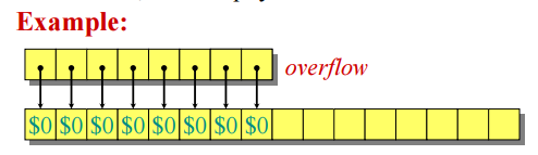
IDEA : Whenever the table gets too full(overflows), “grow” it.

• Allocate(malloc or new) a large table.
• move the items from the old to new.

• Free the old table.

  The aggregate method

  Analysis :
  A sequence of n insertion operations worst-case of 1 insert = O(n)
  let ci = the cost of the i-th insertion = i(if i-1 is an exact power of 2)/ 1(otherwise).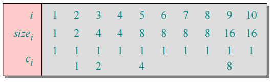
  
  Cost of n insertions =
  
  Thus, the average cost of each dynamic-table operation is O(n)/n= O(1)
  An amortized analysis(平摊分析) is any strategy for analyzing a sequence of operations to show that the average cost per operation is small, even though a single operation within the sequence might be expensive.
  常见的平摊分析技术：

• the aggregate method(聚集分析)

• the accounting method(记账分析)
• the potential method(势能方法)

The aggregate method, though simple, lacks the precision of the other two methods. In particular, the accounting and potential methods allow a specific amortized cost to be allocated to each operation.

The accounting method

• Charge i th operation a fictitious amortized cost ĉ i, where $1 pays for 1 unit of work (i.e., time).
• This fee is consumed to perform the operation.
• Any amount not immediately consumed is stored in the bank for use by subsequent operations.
• The bank balance must not go negative! We must ensure that:

for all n

• Thus, the total amortized costs provide an upper bound on the total true costs.

  Accounting analysis of dynamic tables

  Charge an amortized cost of ĉi = $3 for the i th insertion.

• $1 pays for the immediate insertion.

• $2 is stored for later table doubling.

When the table doubles, $1 pays to move a recent item, and $1 pays to move an old item.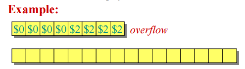


Key invariant : Bank balance never drops below 0. Thus, the sum of the amortized costs provides an upper bound on the sum of the true costs.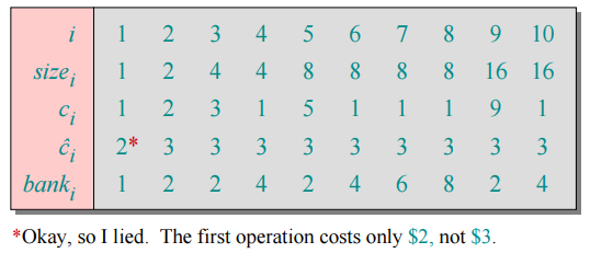

The potential method

IDEA : View the bank account as the potential energy (à la physics) of the dynamic set.
Framework :

• Start with an initial data structure .
• Operation i transforms to .
• The cost of operation i is .
• Define a potenrial function , such that and for all i.
• The amortized cost with respect to Φ is defined to be . 其中，
• if ∆Φi > 0, then ĉi > ci. Operation i stores work in the data structure for later use; If ∆Φi < 0, then ĉi < ci. The data structure delivers up stored work to help pay for operation i.

The total amortized cost of n operations is:

例子略

Conclusions

• Amortized costs can provide a clean abstraction of data-structure performance.
• Any of the analysis methods can be used when an amortized analysis is called for, but each method has some situations where it is arguably the simplest or most precise.
• Different schemes may work for assigning amortized costs in the accounting method, or potentials in the potential method, sometimes yielding radically different bounds.