- Chapter 16. Pig
- Chapter 17. Hive
- Chapter 18. Crunch
- Chapter 19. Spark
- Chapter 20. HBase
- Chapter 21. ZooKeeper
- Installing and Running ZooKeeper
- An Example
- The ZooKeeper Service
- Building Applications with ZooKeeper
- ZooKeeper in Production
- Further Reading
Chapter 16. Pig
Apache Pig raises the level of abstraction for processing large datasets. MapReduce allows you, as the programmer, to specify a map function followed by a reduce function, but working out how to fit your data processing into this pattern, which often requires multiple MapReduce stages, can be a challenge. With Pig, the data structures are much richer, typically being multivalued and nested, and the transformations you can apply to the data are much more powerful. They include joins, for example, which are not for the faint of heart in MapReduce.
Pig is made up of two pieces: The language used to express data flows, called Pig Latin.
The execution environment to run Pig Latin programs. There are currently two environments: local execution in a single JVM and distributed execution on a Hadoop cluster.
A Pig Latin program is made up of a series of operations, or transformations, that are applied to the input data to produce output. Taken as a whole, the operations describe a data flow, which the Pig execution environment translates into an executable representation and then runs. Under the covers, Pig turns the transformations into a series of MapReduce jobs, but as a programmer you are mostly unaware of this, which allows you to focus on the data rather than the nature of the execution.
Pig is a scripting language for exploring large datasets. One criticism of MapReduce is that the development cycle is very long. Writing the mappers and reducers, compiling and packaging the code, submitting the job(s), and retrieving the results is a time-consuming business, and even with Streaming, which removes the compile and package step, the experience is still involved. Pig’s sweet spot is its ability to process terabytes of data in response to a half-dozen lines of Pig Latin issued from the console. Indeed, it was created at Yahoo! to make it easier for researchers and engineers to mine the huge datasets there. Pig is very supportive of a programmer writing a query, since it provides several commands for introspecting the data structures in your program as it is written. Even more useful, it can perform a sample run on a representative subset of your input data, so you can see whether there are errors in the processing before unleashing it on the full dataset.
Pig was designed to be extensible. Virtually all parts of the processing path are customizable: loading, storing, filtering, grouping, and joining can all be altered by userdefined functions (UDFs). These functions operate on Pig’s nested data model, so they can integrate very deeply with Pig’s operators. As another benefit, UDFs tend to be more reusable than the libraries developed for writing MapReduce programs.
In some cases, Pig doesn’t perform as well as programs written in MapReduce. However, the gap is narrowing with each release, as the Pig team implements sophisticated algorithms for applying Pig’s relational operators. It’s fair to say that unless you are willing to invest a lot of effort optimizing Java MapReduce code, writing queries in Pig Latin will save you time.
Installing and Running Pig
Pig runs as a client-side application. Even if you want to run Pig on a Hadoop cluster, there is nothing extra to install on the cluster: Pig launches jobs and interacts with HDFS (or other Hadoop filesystems) from your workstation.
Installation is straightforward. Download a stable release from http://pig.apache.org/releases.html, and unpack the tarball in a suitable place on your workstation:
% tar xzf pig-x.y.z.tar.gz
It’s convenient to add Pig’s binary directory to your command-line path. For example:
% export PIGHOME=~/sw/pig-_x.y.z
% export PATH=$PATH:$PIG_HOME/bin
You also need to set the JAVA_HOME environment variable to point to a suitable Java installation.
Try typing pig -help to get usage instructions.
Execution Types
Pig has two execution types or modes: local mode and MapReduce mode. Execution modes for Apache Tez and Spark (see Chapter 19) were both under development at the time of writing. Both promise significant performance gains over MapReduce mode, so try them if they are available in the version of Pig you are using.
Local mode
In local mode, Pig runs in a single JVM and accesses the local filesystem. This mode is suitable only for small datasets and when trying out Pig.
The execution type is set using the -x or -exectype option. To run in local mode, set the option to local:
% pig -x local grunt>
This starts Grunt, the Pig interactive shell, which is discussed in more detail shortly.
MapReduce mode
In MapReduce mode, Pig translates queries into MapReduce jobs and runs them on a Hadoop cluster. The cluster may be a pseudo- or fully distributed cluster. MapReduce mode (with a fully distributed cluster) is what you use when you want to run Pig on large datasets.
To use MapReduce mode, you first need to check that the version of Pig you downloaded is compatible with the version of Hadoop you are using. Pig releases will only work against particular versions of Hadoop; this is documented in the release notes.
Pig honors the HADOOPHOME environment variable for finding which Hadoop client to run. However, if it is not set, Pig will use a bundled copy of the Hadoop libraries. Note that these may not match the version of Hadoop running on your cluster, so it is best to explicitly set HADOOP_HOME.
Next, you need to point Pig at the cluster’s namenode and resource manager. If the installation of Hadoop at HADOOP_HOME is already configured for this, then there is nothing more to do. Otherwise, you can set HADOOP_CONF_DIR to a directory containing the Hadoop site file (or files) that define fs.defaultFS, yarn.resourcemanager.address, and mapreduce.framework.name (the latter should be set to yarn).
Alternatively, you can set these properties in the _pig.properties file in Pig’s conf directory
(or the directory specified by PIGCONF_DIR). Here’s an example for a pseudo-distributed setup:
fs.defaultFS=hdfs://localhost/ mapreduce.framework.name=yarn yarn.resourcemanager.address=localhost:8032
Once you have configured Pig to connect to a Hadoop cluster, you can launch Pig, setting the -x option to mapreduce or omitting it entirely, as MapReduce mode is the default. We’ve used the -brief option to stop timestamps from being logged:
% pig -brief
Logging error messages to: /Users/tom/pig_1414246949680.log
Default bootup file /Users/tom/.pigbootup not found
Connecting to hadoop file system at: hdfs://localhost/ grunt>
As you can see from the output, Pig reports the filesystem (but not the YARN resource manager) that it has connected to.
In MapReduce mode, you can optionally enable _auto-local mode (by setting pig.auto.local.enabled to true), which is an optimization that runs small jobs locally if the input is less than 100 MB (set by pig.auto.local.input.maxbytes, default 100,000,000) and no more than one reducer is being used.
Running Pig Programs
There are three ways of executing Pig programs, all of which work in both local and MapReduce mode:
Script
Pig can run a script file that contains Pig commands. For example, pig script.pig runs the commands in the local file script.pig. Alternatively, for very short scripts, you can use the -e option to run a script specified as a string on the command line.
Grunt
Grunt is an interactive shell for running Pig commands. Grunt is started when no file is specified for Pig to run and the -e option is not used. It is also possible to run Pig scripts from within Grunt using run and exec.
Embedded
You can run Pig programs from Java using the PigServer class, much like you can use JDBC to run SQL programs from Java. For programmatic access to Grunt, use PigRunner.
Grunt
Grunt has line-editing facilities like those found in GNU Readline (used in the bash shell and many other command-line applications). For instance, the Ctrl-E key combination will move the cursor to the end of the line. Grunt remembers command history, too,96] and you can recall lines in the history buffer using Ctrl-P or Ctrl-N (for previous and next), or equivalently, the up or down cursor keys.
Another handy feature is Grunt’s completion mechanism, which will try to complete Pig Latin keywords and functions when you press the Tab key. For example, consider the following incomplete line: grunt> a = foreach b ge
If you press the Tab key at this point, ge will expand to generate, a Pig Latin keyword: grunt> a = foreach b generate
You can customize the completion tokens by creating a file named autocomplete and placing it on Pig’s classpath (such as in the conf directory in Pig’s install directory) or in the directory you invoked Grunt from. The file should have one token per line, and tokens must not contain any whitespace. Matching is case sensitive. It can be very handy to add commonly used file paths (especially because Pig does not perform filename completion) or the names of any user-defined functions you have created.
You can get a list of commands using the help command. When you’ve finished your Grunt session, you can exit with the quit command, or the equivalent shortcut \q.
Pig Latin Editors
There are Pig Latin syntax highlighters available for a variety of editors, including
Eclipse, IntelliJ IDEA, Vim, Emacs, and TextMate. Details are available on the Pig wiki.
Many Hadoop distributions come with the Hue web interface, which has a Pig script editor and launcher.
An Example
Let’s look at a simple example by writing the program to calculate the maximum recorded
temperature by year for the weather dataset in Pig Latin (just like we did using MapReduce in Chapter 2). The complete program is only a few lines long:
— max_temp.pig: Finds the maximum temperature by year _records = LOAD ‘input/ncdc/micro-tab/sample.txt’
AS (year:chararray, temperature:int, quality:int); filtered_records = FILTER records BY temperature != 9999 AND quality IN (0, 1, 4, 5, 9);
grouped_records = GROUP filtered_records BY year; max_temp = FOREACH grouped_records GENERATE group,
MAX(filtered_records.temperature); DUMP max_temp;
To explore what’s going on, we’ll use Pig’s Grunt interpreter, which allows us to enter lines and interact with the program to understand what it’s doing. Start up Grunt in local mode, and then enter the first line of the Pig script:
grunt> records = LOAD ‘input/ncdc/micro-tab/sample.txt’ >> AS (year:chararray, temperature:int, quality:int);
For simplicity, the program assumes that the input is tab-delimited text, with each line having just year, temperature, and quality fields. (Pig actually has more flexibility than this with regard to the input formats it accepts, as we’ll see later.) This line describes the input data we want to process. The year:chararray notation describes the field’s name and type; chararray is like a Java String, and an int is like a Java int. The LOAD operator takes a URI argument; here we are just using a local file, but we could refer to an HDFS URI. The AS clause (which is optional) gives the fields names to make it convenient to refer to them in subsequent statements.
The result of the LOAD operator, and indeed any operator in Pig Latin, is a _relation, which is just a set of tuples. A tuple is just like a row of data in a database table, with multiple fields in a particular order. In this example, the LOAD function produces a set of (year, temperature, quality) tuples that are present in the input file. We write a relation with one tuple per line, where tuples are represented as comma-separated items in parentheses:
(1950,0,1)
(1950,22,1)
(1950,-11,1)
(1949,111,1)
Relations are given names, or aliases, so they can be referred to. This relation is given the records alias. We can examine the contents of an alias using the DUMP operator:
grunt> DUMP records;
(1950,0,1)
(1950,22,1)
(1950,-11,1)
(1949,111,1) (1949,78,1)
We can also see the structure of a relation — the relation’s schema — using the DESCRIBE operator on the relation’s alias:
grunt> DESCRIBE records; records: {year: chararray,temperature: int,quality: int}
This tells us that records has three fields, with aliases year, temperature, and quality, which are the names we gave them in the AS clause. The fields have the types given to them in the AS clause, too. We examine types in Pig in more detail later.
The second statement removes records that have a missing temperature (indicated by a value of 9999) or an unsatisfactory quality reading. For this small dataset, no records are filtered out:
grunt> filtered_records = FILTER records BY temperature != 9999 AND
>> quality IN (0, 1, 4, 5, 9); grunt> DUMP filtered_records;
(1950,0,1)
(1950,22,1)
(1950,-11,1)
(1949,111,1) (1949,78,1)
The third statement uses the GROUP function to group the records relation by the year field. Let’s use DUMP to see what it produces:
grunt> grouped_records = GROUP filtered_records BY year; grunt> DUMP grouped_records;
(1949,{(1949,78,1),(1949,111,1)})
(1950,{(1950,-11,1),(1950,22,1),(1950,0,1)})
We now have two rows, or tuples: one for each year in the input data. The first field in each tuple is the field being grouped by (the year), and the second field has a bag of tuples for that year. A bag is just an unordered collection of tuples, which in Pig Latin is represented using curly braces.
By grouping the data in this way, we have created a row per year, so now all that remains is to find the maximum temperature for the tuples in each bag. Before we do this, let’s understand the structure of the grouped_records relation:
grunt> DESCRIBE grouped_records;
grouped_records: {group: chararray,filtered_records: {year: chararray, temperature: int,quality: int}}
This tells us that the grouping field is given the alias group by Pig, and the second field is the same structure as the filtered_records relation that was being grouped. With this information, we can try the fourth transformation:
grunt> max_temp = FOREACH grouped_records GENERATE group,
>> MAX(filtered_records.temperature);
FOREACH processes every row to generate a derived set of rows, using a GENERATE clause to define the fields in each derived row. In this example, the first field is group, which is just the year. The second field is a little more complex. The filtered_records.temperature reference is to the temperature field of the filtered_records bag in the grouped_records relation. MAX is a built-in function for calculating the maximum value of fields in a bag. In this case, it calculates the maximum temperature for the fields in each filtered_records bag. Let’s check the result:
grunt> DUMP max_temp;
(1949,111) (1950,22)
We’ve successfully calculated the maximum temperature for each year.
Generating Examples
In this example, we’ve used a small sample dataset with just a handful of rows to make it easier to follow the data flow and aid debugging. Creating a cut-down dataset is an art, as ideally it should be rich enough to cover all the cases to exercise your queries (the completeness property), yet small enough to make sense to the programmer (the conciseness property). Using a random sample doesn’t work well in general because join and filter operations tend to remove all random data, leaving an empty result, which is not illustrative of the general data flow.
With the ILLUSTRATE operator, Pig provides a tool for generating a reasonably complete and concise sample dataset. Here is the output from running ILLUSTRATE on our dataset (slightly reformatted to fit the page):
grunt> ILLUSTRATE max_temp;
———————————————————————————————————————-
| records | year:chararray | temperature:int | quality:int |
———————————————————————————————————————-
| | 1949 | 78 | 1 |
| | 1949 | 111 | 1 |
| | 1949 | 9999 | 1 |
———————————————————————————————————————-
———————————————————————————————————————-
| filtered_records | year:chararray | temperature:int | quality:int |
———————————————————————————————————————-
| | 1949 | 78 | 1 |
| | 1949 | 111 | 1 |
———————————————————————————————————————-
———————————————————————————————————————| grouped_records | group:chararray | filtered_records:bag{:tuple( | year:chararray,temperature:int, | quality:int)} | ———————————————————————————————————————-
| | 1949 | {(1949, 78, 1), (1949, 111, 1)} |
———————————————————————————————————————-
—————————————————————————-
| max_temp | group:chararray | :int |
—————————————————————————-
| | 1949 | 111 |
—————————————————————————-
Notice that Pig used some of the original data (this is important to keep the generated dataset realistic), as well as creating some new data. It noticed the special value 9999 in the query and created a tuple containing this value to exercise the FILTER statement.
In summary, the output of ILLUSTRATE is easy to follow and can help you understand what your query is doing.
Comparison with Databases
Having seen Pig in action, it might seem that Pig Latin is similar to SQL. The presence of such operators as GROUP BY and DESCRIBE reinforces this impression. However, there are several differences between the two languages, and between Pig and relational database management systems (RDBMSs) in general.
The most significant difference is that Pig Latin is a data flow programming language, whereas SQL is a declarative programming language. In other words, a Pig Latin program is a step-by-step set of operations on an input relation, in which each step is a single transformation. By contrast, SQL statements are a set of constraints that, taken together, define the output. In many ways, programming in Pig Latin is like working at the level of an RDBMS query planner, which figures out how to turn a declarative statement into a system of steps.
RDBMSs store data in tables, with tightly predefined schemas. Pig is more relaxed about the data that it processes: you can define a schema at runtime, but it’s optional. Essentially, it will operate on any source of tuples (although the source should support being read in parallel, by being in multiple files, for example), where a UDF is used to read the tuples from their raw representation.97] The most common representation is a text file with tabseparated fields, and Pig provides a built-in load function for this format. Unlike with a traditional database, there is no data import process to load the data into the RDBMS. The data is loaded from the filesystem (usually HDFS) as the first step in the processing.
Pig’s support for complex, nested data structures further differentiates it from SQL, which operates on flatter data structures. Also, Pig’s ability to use UDFs and streaming operators that are tightly integrated with the language and Pig’s nested data structures makes Pig Latin more customizable than most SQL dialects.
RDBMSs have several features to support online, low-latency queries, such as transactions and indexes, that are absent in Pig. Pig does not support random reads or queries on the order of tens of milliseconds. Nor does it support random writes to update small portions of data; all writes are bulk streaming writes, just like with MapReduce.
Hive (covered in Chapter 17) sits between Pig and conventional RDBMSs. Like Pig, Hive is designed to use HDFS for storage, but otherwise there are some significant differences. Its query language, HiveQL, is based on SQL, and anyone who is familiar with SQL will have little trouble writing queries in HiveQL. Like RDBMSs, Hive mandates that all data be stored in tables, with a schema under its management; however, it can associate a schema with preexisting data in HDFS, so the load step is optional. Pig is able to work with Hive tables using HCatalog; this is discussed further in Using Hive tables with HCatalog.
Pig Latin
This section gives an informal description of the syntax and semantics of the Pig Latin programming language.98] It is not meant to offer a complete reference to the language,
[99] but there should be enough here for you to get a good understanding of Pig Latin’s constructs.
Structure
A Pig Latin program consists of a collection of statements. A statement can be thought of as an operation or a command.100] For example, a GROUP operation is a type of statement: groupedrecords = GROUP records BY year;
The command to list the files in a Hadoop filesystem is another example of a statement: ls /
Statements are usually terminated with a semicolon, as in the example of the GROUP statement. In fact, this is an example of a statement that must be terminated with a semicolon; it is a syntax error to omit it. The ls command, on the other hand, does not have to be terminated with a semicolon. As a general guideline, statements or commands for interactive use in Grunt do not need the terminating semicolon. This group includes the interactive Hadoop commands, as well as the diagnostic operators such as DESCRIBE. It’s never an error to add a terminating semicolon, so if in doubt, it’s simplest to add one.
Statements that have to be terminated with a semicolon can be split across multiple lines for readability:
records = LOAD ‘input/ncdc/micro-tab/sample.txt’ AS (year:chararray, temperature:int, quality:int);
Pig Latin has two forms of comments. Double hyphens are used for single-line comments. Everything from the first hyphen to the end of the line is ignored by the Pig Latin interpreter:
— My program
DUMP A; — What’s in A?
C-style comments are more flexible since they delimit the beginning and end of the comment block with / and / markers. They can span lines or be embedded in a single line:
/ _
Description of my program spanning
multiple lines.
_/
A = LOAD ‘input/pig/join/A’;
B = LOAD ‘input/pig/join/B’;
C = JOIN A BY $0, / ignored /_ B BY $1; DUMP C;
Pig Latin has a list of keywords that have a special meaning in the language and cannot be used as identifiers. These include the operators (LOAD, ILLUSTRATE), commands (cat, ls), expressions (matches, FLATTEN), and functions (DIFF, MAX) — all of which are covered in the following sections.
Pig Latin has mixed rules on case sensitivity. Operators and commands are not case sensitive (to make interactive use more forgiving); however, aliases and function names are case sensitive.
Statements
As a Pig Latin program is executed, each statement is parsed in turn. If there are syntax errors or other (semantic) problems, such as undefined aliases, the interpreter will halt and display an error message. The interpreter builds a logical plan for every relational operation, which forms the core of a Pig Latin program. The logical plan for the statement is added to the logical plan for the program so far, and then the interpreter moves on to the next statement.
It’s important to note that no data processing takes place while the logical plan of the program is being constructed. For example, consider again the Pig Latin program from the first example:
— max_temp.pig: Finds the maximum temperature by year _records = LOAD ‘input/ncdc/micro-tab/sample.txt’
AS (year:chararray, temperature:int, quality:int); filtered_records = FILTER records BY temperature != 9999 AND quality IN (0, 1, 4, 5, 9);
grouped_records = GROUP filtered_records BY year; max_temp = FOREACH grouped_records GENERATE group,
MAX(filtered_records.temperature);
DUMP max_temp;
When the Pig Latin interpreter sees the first line containing the LOAD statement, it confirms that it is syntactically and semantically correct and adds it to the logical plan, but it does not load the data from the file (or even check whether the file exists). Indeed, where would it load it? Into memory? Even if it did fit into memory, what would it do with the data? Perhaps not all the input data is needed (because later statements filter it, for example), so it would be pointless to load it. The point is that it makes no sense to start any processing until the whole flow is defined. Similarly, Pig validates the GROUP and FOREACH…GENERATE statements, and adds them to the logical plan without executing them. The trigger for Pig to start execution is the DUMP statement. At that point, the logical plan is compiled into a physical plan and executed.
MULTIQUERY EXECUTION Because DUMP is a diagnostic tool, it will always trigger execution. However, the STORE command is different. In interactive mode, STORE acts like DUMP and will always trigger execution (this includes the run command), but in batch mode it will not (this includes the exec command). The reason for this is efficiency. In batch mode, Pig will parse the whole script to see whether there are any optimizations that could be made to limit the amount of data to be written to or read from disk. Consider the following simple example:
A = LOAD ‘input/pig/multiquery/A’;
B = FILTER A BY $1 == ‘banana’;
C = FILTER A BY $1 != ‘banana’;
STORE B INTO ‘output/b’;
STORE C INTO ‘output/c’;
Relations B and C are both derived from A, so to save reading A twice, Pig can run this script as a single MapReduce job by reading A once and writing two output files from the job, one for each of B and C. This feature is called _multiquery execution.
In previous versions of Pig that did not have multiquery execution, each STORE statement in a script run in batch mode triggered execution, resulting in a job for each STORE statement. It is possible to restore the old behavior by disabling multiquery execution with the -M or -nomultiquery option to pig.
The physical plan that Pig prepares is a series of MapReduce jobs, which in local mode Pig runs in the local JVM and in MapReduce mode Pig runs on a Hadoop cluster.
NOTE
You can see the logical and physical plans created by Pig using the EXPLAIN command on a relation (EXPLAIN max_temp;, for example). EXPLAIN will also show the MapReduce plan, which shows how the physical operators are grouped into MapReduce jobs. This is a good way to find out how many MapReduce jobs Pig will run for your query.
The relational operators that can be a part of a logical plan in Pig are summarized in
Table 16-1. We go through the operators in more detail in Data Processing Operators.
_Table 16-1. Pig Latin relational operators
Category Operator Description
Loading and storing LOAD Loads data from the filesystem or other storage into a relation
| STORE | Saves a relation to the filesystem or other storage | |
|---|---|---|
DUMP (\d) Prints a relation to the console
| Filtering | FILTER | Removes unwanted rows from a relation |
|---|---|---|
| DISTINCT | Removes duplicate rows from a relation | |
| FOREACH… GENERATE |
Adds or removes fields to or from a relation | |
| MAPREDUCE | Runs a MapReduce job using a relation as input | |
| STREAM | Transforms a relation using an external program | |
| SAMPLE | Selects a random sample of a relation | |
| ASSERT | Ensures a condition is true for all rows in a relation; otherwise, fails |
Grouping and joining JOIN Joins two or more relations
| COGROUP | Groups the data in two or more relations |
|---|---|
| GROUP | Groups the data in a single relation |
| CROSS | Creates the cross product of two or more relations |
CUBE Creates aggregations for all combinations of specified columns in a relation
| Sorting | ORDER | Sorts a relation by one or more fields |
|---|---|---|
| RANK | Assign a rank to each tuple in a relation, optionally sorting by fields first | |
| LIMIT | Limits the size of a relation to a maximum number of tuples |
 Combining and UNION splitting
There are other types of statements that are not added to the logical plan. For example, the diagnostic operators — DESCRIBE, EXPLAIN, and ILLUSTRATE — are provided to allow the user to interact with the logical plan for debugging purposes (see Table 16-2). DUMP is a sort of diagnostic operator, too, since it is used only to allow interactive debugging of small result sets or in combination with LIMIT to retrieve a few rows from a larger relation. The STORE statement should be used when the size of the output is more than a few lines, as it writes to a file rather than to the console.
Table 16-2. Pig Latin diagnostic operators
Operator (Shortcut) Description
| DESCRIBE (\de) | Prints a relation’s schema |
|---|---|
| EXPLAIN (\e) | Prints the logical and physical plans |
| ILLUSTRATE (\i) | Shows a sample execution of the logical plan, using a generated subset of the input |
Pig Latin also provides three statements — REGISTER, DEFINE, and IMPORT — that make it possible to incorporate macros and user-defined functions into Pig scripts (see Table 163).
Table 16-3. Pig Latin macro and UDF statements
Statement Description
| REGISTER | Registers a JAR file with the Pig runtime |
|---|---|
| DEFINE | Creates an alias for a macro, UDF, streaming script, or command specification |
| IMPORT | Imports macros defined in a separate file into a script |
Because they do not process relations, commands are not added to the logical plan; instead, they are executed immediately. Pig provides commands to interact with Hadoop filesystems (which are very handy for moving data around before or after processing with Pig) and MapReduce, as well as a few utility commands (described in Table 16-4).
Table 16-4. Pig Latin commands
Category Command Description
Hadoop filesystem cat Prints the contents of one or more files
| cd | Changes the current directory |
|---|---|
copyFromLocal Copies a local file or directory to a Hadoop filesystem
| copyToLocal | Copies a file or directory on a Hadoop filesystem to the local filesystem | |
|---|---|---|
| cp | Copies a file or directory to another directory | |
| fs | Accesses Hadoop’s filesystem shell | |
| ls | Lists files | |
| mkdir | Creates a new directory | |
| mv | Moves a file or directory to another directory | |
| pwd | Prints the path of the current working directory | |
| rm | Deletes a file or directory | |
| rmf | Forcibly deletes a file or directory (does not fail if the file or directory does not exist) |
Hadoop kill Kills a MapReduce job
MapReduce
| Utility | clear | Clears the screen in Grunt |
|---|---|---|
| exec | Runs a script in a new Grunt shell in batch mode | |
| help | Shows the available commands and options | |
| history | Prints the query statements run in the current Grunt session | |
| quit (\q) | Exits the interpreter | |
| run | Runs a script within the existing Grunt shell | |
| set | Sets Pig options and MapReduce job properties | |
| sh | Runs a shell command from within Grunt |
The filesystem commands can operate on files or directories in any Hadoop filesystem, and they are very similar to the hadoop fs commands (which is not surprising, as both are simple wrappers around the Hadoop FileSystem interface). You can access all of the Hadoop filesystem shell commands using Pig’s fs command. For example, fs -ls will show a file listing, and fs -help will show help on all the available commands.
Precisely which Hadoop filesystem is used is determined by the fs.defaultFS property in the site file for Hadoop Core. See The Command-Line Interface for more details on how to configure this property.
These commands are mostly self-explanatory, except set, which is used to set options that control Pig’s behavior (including arbitrary MapReduce job properties). The debug option is used to turn debug logging on or off from within a script (you can also control the log level when launching Pig, using the -d or -debug option): grunt> set debug on
Another useful option is the job.name option, which gives a Pig job a meaningful name, making it easier to pick out your Pig MapReduce jobs when running on a shared Hadoop cluster. If Pig is running a script (rather than operating as an interactive query from Grunt), its job name defaults to a value based on the script name.
There are two commands in Table 16-4 for running a Pig script, exec and run. The difference is that exec runs the script in batch mode in a new Grunt shell, so any aliases defined in the script are not accessible to the shell after the script has completed. On the other hand, when running a script with run, it is as if the contents of the script had been entered manually, so the command history of the invoking shell contains all the statements from the script. Multiquery execution, where Pig executes a batch of statements in one go (see Multiquery Execution), is used only by exec, not run.
CONTROL FLOW By design, Pig Latin lacks native control flow statements. The recommended approach for writing programs that have conditional logic or loop constructs is to embed Pig Latin in another language, such as Python, JavaScript, or Java, and manage the control flow from there. In this model, the host script uses a compile-bind-run API to execute Pig scripts and retrieve their status. Consult the Pig documentation for details of the API.
Embedded Pig programs always run in a JVM, so for Python and JavaScript you use the pig command followed by the name of your script, and the appropriate Java scripting engine will be selected (Jython for Python, Rhino for JavaScript).
Expressions
An expression is something that is evaluated to yield a value. Expressions can be used in Pig as a part of a statement containing a relational operator. Pig has a rich variety of expressions, many of which will be familiar from other programming languages. They are listed in Table 16-5, with brief descriptions and examples. We will see examples of many of these expressions throughout the chapter.
Table 16-5. Pig Latin expressions
| Category | Expressions | Description | Examples |
|---|---|---|---|
| Constant | Literal | Constant value (see also the “Literal example” column in Table 16-6) | 1.0, ‘a’ |
| Field (by position) | $n | Field in position n (zero-based) | $0 |
| Field (by name) | f | Field named f | year |
| Field (disambiguate) |
r::f | Field named f from relation r after grouping or joining | A::year |
| Projection | c.$n, c.f | Field in container c (relation, bag, or tuple) by position, by name | records.$0, records.year |
| Map lookup | m#k | Value associated with key k in map m | items#’Coat’ |
Cast () Cast of field f to type t (int) year
| Arithmetic | x + y, x - y | Addition, subtraction | $1 + $2, $1 - $2 |
|---|---|---|---|
| x * y, x / y | Multiplication, division | $1 * $2, $1 / $2 | |
| x % y | Modulo, the remainder of x divided by y | $1 % $2 | |
| +x, -x | Unary positive, negation | +1, –1 | |
| Conditional | x ? y : z | Bincond/ternary; y if x evaluates to true, _z _otherwise | quality == 0 ? 0 : 1 |
| CASE | Multi-case conditional | CASE q WHEN 0 THEN ‘good’ ELSE ‘bad’ END |
|
| Comparison | x == y, x != y |
Equals, does not equal | quality == 0, temperature != 9999 |
| x > y, x < y | Greater than, less than | quality > 0, quality < 10 | |
| x >= y, x <= y |
Greater than or equal to, less than or equal to | quality >= 1, quality <= 9 | |
| x matches y | Pattern matching with regular expression | quality matches ‘[01459]’ | |
| x is null | Is null | temperature is null | |
| x is not null | Is not null | temperature is not null | |
| Boolean | x OR y | Logical OR | q == 0 OR q == 1 |
| x AND y | Logical AND | q == 0 AND r == 0 | |
| NOT x | Logical negation | NOT q matches ‘[01459]’ | |
| IN x | Set membership | q IN (0, 1, 4, 5, 9) | |
| Functional | fn(,,…) Invocation of function fn on fields f1, f2, etc. | isGood(quality) |
Flatten FLATTEN(__) Removal of a level of nesting from bags and tuples FLATTEN(group)
Types
So far you have seen some of the simple types in Pig, such as int and chararray. Here we will discuss Pig’s built-in types in more detail.
Pig has a boolean type and six numeric types: int, long, float, double, biginteger, and bigdecimal, which are identical to their Java counterparts. There is also a bytearray type, like Java’s byte array type for representing a blob of binary data, and chararray, which, like java.lang.String, represents textual data in UTF-16 format (although it can be loaded or stored in UTF-8 format). The datetime type is for storing a date and time with millisecond precision and including a time zone.
Pig does not have types corresponding to Java’s byte, short, or char primitive types. These are all easily represented using Pig’s int type, or chararray for char.
The Boolean, numeric, textual, binary, and temporal types are simple atomic types. Pig Latin also has three complex types for representing nested structures: tuple, bag, and map. All of Pig Latin’s types are listed in Table 16-6.
Table 16-6. Pig Latin types
Category Type Description Literal example
Boolean boolean True/false value true
| Numeric | int | 32-bit signed integer | 1 | |
|---|---|---|---|---|
| long | 64-bit signed integer | 1L | ||
| float | 32-bit floating-point number | 1.0F | ||
| double | 64-bit floating-point number | 1.0 | ||
| biginteger | Arbitrary-precision integer | ‘10000000000’ | ||
| bigdecimal | Arbitrary-precision signed decimal number | ‘0.110001000000000000000001’ | ||
| Text | chararray | Character array in UTF-16 format | ‘a’ |
Binary bytearray Byte array Not supported
| Temporal datetime | Date and time with time zone | Not supported, use ToDate builtin function | |
|---|---|---|---|
| Complex | tuple | Sequence of fields of any type | (1,’pomegranate’) |
| bag | Unordered collection of tuples, possibly with duplicates | {(1,’pomegranate’),(2)} | |
| map | Set of key-value pairs; keys must be character arrays, but values may be any type | [‘a’#’pomegranate’] |
The complex types are usually loaded from files or constructed using relational operators. Be aware, however, that the literal form in Table 16-6 is used when a constant value is created from within a Pig Latin program. The raw form in a file is usually different when using the standard PigStorage loader. For example, the representation in a file of the bag in Table 16-6 would be {(1,pomegranate),(2)} (note the lack of quotation marks), and with a suitable schema, this would be loaded as a relation with a single field and row, whose value was the bag.
Pig provides the built-in functions TOTUPLE, TOBAG, and TOMAP, which are used for turning expressions into tuples, bags, and maps.
Although relations and bags are conceptually the same (unordered collections of tuples), in practice Pig treats them slightly differently. A relation is a top-level construct, whereas a bag has to be contained in a relation. Normally you don’t have to worry about this, but there are a few restrictions that can trip up the uninitiated. For example, it’s not possible to create a relation from a bag literal. So, the following statement fails:
A = {(1,2),(3,4)};—Error
The simplest workaround in this case is to load the data from a file using the LOAD statement.
As another example, you can’t treat a relation like a bag and project a field into a new relation ($0 refers to the first field of A, using the positional notation):
B = A.$0;
Instead, you have to use a relational operator to turn the relation A into relation B:
B = FOREACH A GENERATE $0;
It’s possible that a future version of Pig Latin will remove these inconsistencies and treat relations and bags in the same way.
Schemas
A relation in Pig may have an associated schema, which gives the fields in the relation names and types. We’ve seen how an AS clause in a LOAD statement is used to attach a schema to a relation:
grunt> records = LOAD ‘input/ncdc/micro-tab/sample.txt’
>> AS (year:int, temperature:int, quality:int); grunt> DESCRIBE records; records: {year: int,temperature: int,quality: int}
This time we’ve declared the year to be an integer rather than a chararray, even though the file it is being loaded from is the same. An integer may be more appropriate if we need to manipulate the year arithmetically (to turn it into a timestamp, for example), whereas the chararray representation might be more appropriate when it’s being used as a simple identifier. Pig’s flexibility in the degree to which schemas are declared contrasts with schemas in traditional SQL databases, which are declared before the data is loaded into the system. Pig is designed for analyzing plain input files with no associated type information, so it is quite natural to choose types for fields later than you would with an RDBMS.
It’s possible to omit type declarations completely, too:
grunt> records = LOAD ‘input/ncdc/micro-tab/sample.txt’
>> AS (year, temperature, quality); grunt> DESCRIBE records; records: {year: bytearray,temperature: bytearray,quality: bytearray}
In this case, we have specified only the names of the fields in the schema: year, temperature, and quality. The types default to bytearray, the most general type, representing a binary string.
You don’t need to specify types for every field; you can leave some to default to bytearray, as we have done for year in this declaration:
grunt> records = LOAD ‘input/ncdc/micro-tab/sample.txt’
>> AS (year, temperature:int, quality:int); grunt> DESCRIBE records; records: {year: bytearray,temperature: int,quality: int}
However, if you specify a schema in this way, you do need to specify every field. Also, there’s no way to specify the type of a field without specifying the name. On the other hand, the schema is entirely optional and can be omitted by not specifying an AS clause:
grunt> records = LOAD ‘input/ncdc/micro-tab/sample.txt’; grunt> DESCRIBE records;
Schema for records unknown.
Fields in a relation with no schema can be referenced using only positional notation: $0 refers to the first field in a relation, $1 to the second, and so on. Their types default to bytearray:
grunt> projected_records = FOREACH records GENERATE $0, $1, $2; grunt> DUMP projected_records;
(1950,0,1)
(1950,22,1)
(1950,-11,1)
(1949,111,1) (1949,78,1)
grunt> DESCRIBE projected_records; projected_records: {bytearray,bytearray,bytearray}
Although it can be convenient not to assign types to fields (particularly in the first stages of writing a query), doing so can improve the clarity and efficiency of Pig Latin programs and is generally recommended.
Using Hive tables with HCatalog
Declaring a schema as a part of the query is flexible but doesn’t lend itself to schema reuse. A set of Pig queries over the same input data will often have the same schema repeated in each query. If the query processes a large number of fields, this repetition can become hard to maintain.
HCatalog (which is a component of Hive) solves this problem by providing access to Hive’s metastore, so that Pig queries can reference schemas by name, rather than specifying them in full each time. For example, after running through An Example to load data into a Hive table called records, Pig can access the table’s schema and data as follows:
% pig -useHCatalog
grunt> records = LOAD ‘records’ USING org.apache.hcatalog.pig.HCatLoader(); grunt> DESCRIBE records;
records: {year: chararray,temperature: int,quality: int} grunt> DUMP records;
(1950,0,1)
(1950,22,1)
(1950,-11,1)
(1949,111,1)
(1949,78,1)
Validation and nulls
A SQL database will enforce the constraints in a table’s schema at load time; for example, trying to load a string into a column that is declared to be a numeric type will fail. In Pig, if the value cannot be cast to the type declared in the schema, it will substitute a null value. Let’s see how this works when we have the following input for the weather data, which has an “e” character in place of an integer:
1950 0 1
1950 22 1
1950 e 1
1949 111 1
1949 78 1
Pig handles the corrupt line by producing a null for the offending value, which is displayed as the absence of a value when dumped to screen (and also when saved using STORE):
grunt> records = LOAD ‘input/ncdc/micro-tab/sample_corrupt.txt’
>> AS (year:chararray, temperature:int, quality:int); grunt> DUMP records;
(1950,0,1)
(1950,22,1)
(1950,,1)
(1949,111,1) (1949,78,1)
Pig produces a warning for the invalid field (not shown here) but does not halt its processing. For large datasets, it is very common to have corrupt, invalid, or merely unexpected data, and it is generally infeasible to incrementally fix every unparsable record. Instead, we can pull out all of the invalid records in one go so we can take action on them, perhaps by fixing our program (because they indicate that we have made a mistake) or by filtering them out (because the data is genuinely unusable):
grunt> corrupt_records = FILTER records BY temperature is null; grunt> DUMP corrupt_records; (1950,,1)
Note the use of the is null operator, which is analogous to SQL. In practice, we would include more information from the original record, such as an identifier and the value that could not be parsed, to help our analysis of the bad data.
We can find the number of corrupt records using the following idiom for counting the number of rows in a relation:
grunt> grouped = GROUP corrupt_records ALL;
grunt> all_grouped = FOREACH grouped GENERATE group, COUNT(corrupt_records); grunt> DUMP all_grouped;
(all,1)
(GROUP explains grouping and the ALL operation in more detail.)
Another useful technique is to use the SPLIT operator to partition the data into “good” and “bad” relations, which can then be analyzed separately:
grunt> SPLIT records INTO good_records IF temperature is not null,
>> bad_records OTHERWISE; grunt> DUMP good_records;
(1950,0,1)
(1950,22,1)
(1949,111,1) (1949,78,1) grunt> DUMP bad_records; (1950,,1)
Going back to the case in which temperature’s type was left undeclared, the corrupt data cannot be detected easily, since it doesn’t surface as a null:
grunt> records = LOAD ‘input/ncdc/micro-tab/sample_corrupt.txt’
>> AS (year:chararray, temperature, quality:int); grunt> DUMP records;
(1950,0,1)
(1950,22,1)
(1950,e,1)
(1949,111,1) (1949,78,1) grunt> filtered_records = FILTER records BY temperature != 9999 AND
>> quality IN (0, 1, 4, 5, 9);
grunt> grouped_records = GROUP filtered_records BY year; grunt> max_temp = FOREACH grouped_records GENERATE group,
>> MAX(filtered_records.temperature); grunt> DUMP max_temp;
(1949,111.0) (1950,22.0)
What happens in this case is that the temperature field is interpreted as a bytearray, so the corrupt field is not detected when the input is loaded. When passed to the MAX function, the temperature field is cast to a double, since MAX works only with numeric types. The corrupt field cannot be represented as a double, so it becomes a null, which MAX silently ignores. The best approach is generally to declare types for your data on loading and look for missing or corrupt values in the relations themselves before you do your main processing.
Sometimes corrupt data shows up as smaller tuples because fields are simply missing. You can filter these out by using the SIZE function as follows:
grunt> A = LOAD ‘input/pig/corrupt/missing_fields’; grunt> DUMP A;
(2,Tie)
(4,Coat)
(3) (1,Scarf)
grunt> B = FILTER A BY SIZE(TOTUPLE(*)) > 1; grunt> DUMP B;
(2,Tie)
(4,Coat)
(1,Scarf)
Schema merging
In Pig, you don’t declare the schema for every new relation in the data flow. In most cases, Pig can figure out the resulting schema for the output of a relational operation by considering the schema of the input relation.
How are schemas propagated to new relations? Some relational operators don’t change the schema, so the relation produced by the LIMIT operator (which restricts a relation to a maximum number of tuples), for example, has the same schema as the relation it operates on. For other operators, the situation is more complicated. UNION, for example, combines two or more relations into one and tries to merge the input relations’ schemas. If the schemas are incompatible, due to different types or number of fields, then the schema of the result of the UNION is unknown.
You can find out the schema for any relation in the data flow using the DESCRIBE operator. If you want to redefine the schema for a relation, you can use the FOREACH…GENERATE operator with AS clauses to define the schema for some or all of the fields of the input relation.
See User-Defined Functions for a further discussion of schemas.
Functions
Functions in Pig come in four types:
Eval function
A function that takes one or more expressions and returns another expression. An example of a built-in eval function is MAX, which returns the maximum value of the entries in a bag. Some eval functions are aggregate functions, which means they operate on a bag of data to produce a scalar value; MAX is an example of an aggregate function. Furthermore, many aggregate functions are algebraic, which means that the result of the function may be calculated incrementally. In MapReduce terms, algebraic functions make use of the combiner and are much more efficient to calculate (see Combiner Functions). MAX is an algebraic function, whereas a function to calculate the median of a collection of values is an example of a function that is not algebraic.
Filter function
A special type of eval function that returns a logical Boolean result. As the name suggests, filter functions are used in the FILTER operator to remove unwanted rows. They can also be used in other relational operators that take Boolean conditions, and in general, in expressions using Boolean or conditional expressions. An example of a built-in filter function is IsEmpty, which tests whether a bag or a map contains any items.
Load function
A function that specifies how to load data into a relation from external storage.
Store function
A function that specifies how to save the contents of a relation to external storage.
Often, load and store functions are implemented by the same type. For example, PigStorage, which loads data from delimited text files, can store data in the same format.
Pig comes with a collection of built-in functions, a selection of which are listed in Table 16-7. The complete list of built-in functions, which includes a large number of standard math, string, date/time, and collection functions, can be found in the documentation for each Pig release.
_Table 16-7. A selection of Pig’s built-in functions _Category Function Description
| Eval | AVG | Calculates the average (mean) value of entries in a bag. |
|---|---|---|
| CONCAT | Concatenates byte arrays or character arrays together. | |
| COUNT | Calculates the number of non-null entries in a bag. | |
| COUNT_STAR | Calculates the number of entries in a bag, including those that are null. | |
| DIFF | Calculates the set difference of two bags. If the two arguments are not bags, returns a bag containing both if they are equal; otherwise, returns an empty bag. | |
| MAX | Calculates the maximum value of entries in a bag. | |
| MIN | Calculates the minimum value of entries in a bag. | |
| SIZE | Calculates the size of a type. The size of numeric types is always 1; for character arrays, it is the number of characters; for byte arrays, the number of bytes; and for containers (tuple, bag, map), it is the number of entries. | |
| SUM | Calculates the sum of the values of entries in a bag. | |
| TOBAG | Converts one or more expressions to individual tuples, which are then put in a bag. A synonym for (). | |
| TOKENIZE | Tokenizes a character array into a bag of its constituent words. | |
| TOMAP | Converts an even number of expressions to a map of key-value pairs. A synonym for []. | |
| TOP | Calculates the top n tuples in a bag. | |
| TOTUPLE | Converts one or more expressions to a tuple. A synonym for {}. |
Filter IsEmpty Tests whether a bag or map is empty.
| Load/Store PigStorage | Loads or stores relations using a field-delimited text format. Each line is broken into fields using a configurable field delimiter (defaults to a tab character) to be stored in the tuple’s fields. It is the default storage when none is specified.[a] | |
|---|---|---|
| TextLoader | Loads relations from a plain-text format. Each line corresponds to a tuple whose single field is the line of text. | |
| JsonLoader, JsonStorage |
Loads or stores relations from or to a (Pig-defined) JSON format. Each tuple is stored on one line. | |
| AvroStorage | Loads or stores relations from or to Avro datafiles. | |
| ParquetLoader, ParquetStorer |
Loads or stores relations from or to Parquet files. | |
| OrcStorage | Loads or stores relations from or to Hive ORCFiles. | |
| HBaseStorage | Loads or stores relations from or to HBase tables. |
[a] The default storage can be changed by setting pig.default.load.func and pig.default.store.func to the fully qualified load and store function classnames.
Other libraries
If the function you need is not available, you can write your own user-defined function (or UDF for short), as explained in User-Defined Functions. Before you do that, however, have a look in the Piggy Bank, a library of Pig functions shared by the Pig community and distributed as a part of Pig. For example, there are load and store functions in the Piggy Bank for CSV files, Hive RCFiles, sequence files, and XML files. The Piggy Bank JAR file comes with Pig, and you can use it with no further configuration. Pig’s API documentation includes a list of functions provided by the Piggy Bank.
Apache DataFu is another rich library of Pig UDFs. In addition to general utility functions, it includes functions for computing basic statistics, performing sampling and estimation, hashing, and working with web data (sessionization, link analysis).
Macros
Macros provide a way to package reusable pieces of Pig Latin code from within Pig Latin itself. For example, we can extract the part of our Pig Latin program that performs grouping on a relation and then finds the maximum value in each group by defining a macro as follows:
DEFINE max_by_group(X, group_key, max_field) RETURNS Y {
A = GROUP $X by $group_key;
$Y = FOREACH A GENERATE group, MAX($X.$max_field); };
The macro, called max_by_group, takes three parameters: a relation, X, and two field names, group_key and max_field. It returns a single relation, Y. Within the macro body, parameters and return aliases are referenced with a $ prefix, such as $X.
The macro is used as follows:
records = LOAD ‘input/ncdc/micro-tab/sample.txt’ AS (year:chararray, temperature:int, quality:int); filtered_records = FILTER records BY temperature != 9999 AND quality IN (0, 1, 4, 5, 9); max_temp = **max_by_group(filtered_records, year, temperature); DUMP max_temp
At runtime, Pig will expand the macro using the macro definition. After expansion, the program looks like the following, with the expanded section in bold:
records = LOAD ‘input/ncdc/micro-tab/sample.txt’ AS (year:chararray, temperature:int, quality:int); filtered_records = FILTER records BY temperature != 9999 AND quality IN (0, 1, 4, 5, 9);
macro_max_by_group_A_0 = GROUP filtered_records by (year); max_temp = FOREACH macro_max_by_group_A_0 GENERATE group,
MAX(filtered_records.(temperature)); DUMP max_temp
Normally you don’t see the expanded form, because Pig creates it internally; however, in some cases it is useful to see it when writing and debugging macros. You can get Pig to perform macro expansion only (without executing the script) by passing the -dryrun argument to pig.
Notice that the parameters that were passed to the macro (filtered_records, year, and temperature) have been substituted for the names in the macro definition. Aliases in the macro definition that don’t have a $ prefix, such as A in this example, are local to the macro definition and are rewritten at expansion time to avoid conflicts with aliases in other parts of the program. In this case, A becomes macro_max_by_group_A_0 in the expanded form.
To foster reuse, macros can be defined in separate files to Pig scripts, in which case they need to be imported into any script that uses them. An import statement looks like this:
IMPORT** ‘./ch16-pig/src/main/pig/max_temp.macro’;
User-Defined Functions
Pig’s designers realized that the ability to plug in custom code is crucial for all but the most trivial data processing jobs. For this reason, they made it easy to define and use userdefined functions. We only cover Java UDFs in this section, but be aware that you can also write UDFs in Python, JavaScript, Ruby, or Groovy, all of which are run using the Java Scripting API.
A Filter UDF
Let’s demonstrate by writing a filter function for filtering out weather records that do not have a temperature quality reading of satisfactory (or better). The idea is to change this line:
filtered_records = FILTER records BY temperature != 9999 AND quality IN (0, 1, 4, 5, 9);
to: filtered_records = FILTER records BY temperature != 9999 AND isGood(quality);
This achieves two things: it makes the Pig script a little more concise, and it encapsulates the logic in one place so that it can be easily reused in other scripts. If we were just writing an ad hoc query, we probably wouldn’t bother to write a UDF. It’s when you start doing the same kind of processing over and over again that you see opportunities for reusable UDFs.
Filter UDFs are all subclasses of FilterFunc, which itself is a subclass of EvalFunc. We’ll look at EvalFunc in more detail later, but for the moment just note that, in essence, EvalFunc looks like the following class:
public abstract class EvalFunc
EvalFunc’s only abstract method, exec(), takes a tuple and returns a single value, the (parameterized) type T. The fields in the input tuple consist of the expressions passed to the function — in this case, a single integer. For FilterFunc, T is Boolean, so the method should return true only for those tuples that should not be filtered out.
For the quality filter, we write a class, IsGoodQuality, that extends FilterFunc and implements the exec() method (see Example 16-1). The Tuple class is essentially a list of objects with associated types. Here we are concerned only with the first field (since the function only has a single argument), which we extract by index using the get() method on Tuple. The field is an integer, so if it’s not null, we cast it and check whether the value is one that signifies the temperature was a good reading, returning the appropriate value, true or false.
Example 16-1. A FilterFunc UDF to remove records with unsatisfactory temperature quality readings
package com.hadoopbook.pig;
import java.io.IOException; import java.util.ArrayList; import java.util.List; import org.apache.pig.FilterFunc; import org.apache.pig.backend.executionengine.ExecException; import org.apache.pig.data.DataType; import org.apache.pig.data.Tuple;
import org.apache.pig.impl.logicalLayer.FrontendException; public class IsGoodQuality extends FilterFunc {
@Override
public Boolean exec(Tuple tuple) throws IOException { if (tuple == null || tuple.size() == 0) { return false;
} try {
Object object = tuple.get(0); if (object == null) { return false;
}
int i = (Integer) object; return i == 0 || i == 1 || i == 4 || i == 5 || i == 9;
} catch (ExecException e) { throw new IOException(e);
}
}
}
To use the new function, we first compile it and package it in a JAR file (the example code that accompanies this book comes with build instructions for how to do this). Then we tell Pig about the JAR file with the REGISTER operator, which is given the local path to the filename (and is not enclosed in quotes): grunt> REGISTER pig-examples.jar;
Finally, we can invoke the function:
grunt> filtered_records = FILTER records BY temperature != 9999 AND
>> com.hadoopbook.pig.IsGoodQuality(quality);
Pig resolves function calls by treating the function’s name as a Java classname and attempting to load a class of that name. (This, incidentally, is why function names are case sensitive: because Java classnames are.) When searching for classes, Pig uses a classloader that includes the JAR files that have been registered. When running in distributed mode, Pig will ensure that your JAR files get shipped to the cluster.
For the UDF in this example, Pig looks for a class with the name com.hadoopbook.pig.IsGoodQuality, which it finds in the JAR file we registered.
Resolution of built-in functions proceeds in the same way, except for one difference: Pig has a set of built-in package names that it searches, so the function call does not have to be a fully qualified name. For example, the function MAX is actually implemented by a class MAX in the package org.apache.pig.builtin. This is one of the packages that Pig looks in, so we can write MAX rather than org.apache.pig.builtin.MAX in our Pig programs.
We can add our package name to the search path by invoking Grunt with this commandline argument: -Dudf.import.list=com.hadoopbook.pig. Alternatively, we can shorten the function name by defining an alias, using the DEFINE operator:
grunt> DEFINE isGood com.hadoopbook.pig.IsGoodQuality();
grunt> filtered_records = FILTER records BY temperature != 9999 AND >> isGood(quality);
Defining an alias is a good idea if you want to use the function several times in the same script. It’s also necessary if you want to pass arguments to the constructor of the UDF’s implementation class.
Leveraging types
The filter works when the quality field is declared to be of type int, but if the type information is absent, the UDF fails! This happens because the field is the default type, bytearray, represented by the DataByteArray class. Because DataByteArray is not an Integer, the cast fails.
The obvious way to fix this is to convert the field to an integer in the exec() method. However, there is a better way, which is to tell Pig the types of the fields that the function expects. The getArgToFuncMapping() method on EvalFunc is provided for precisely this reason. We can override it to tell Pig that the first field should be an integer:
@Override
public List
return funcSpecs; }
This method returns a FuncSpec object corresponding to each of the fields of the tuple that are passed to the exec() method. Here there is a single field, and we construct an anonymous FieldSchema (the name is passed as null, since Pig ignores the name when doing type conversion). The type is specified using the INTEGER constant on Pig’s DataType class.
With the amended function, Pig will attempt to convert the argument passed to the function to an integer. If the field cannot be converted, then a null is passed for the field.
The exec() method always returns false when the field is null. For this application, this behavior is appropriate, as we want to filter out records whose quality field is unintelligible.
An Eval UDF
Writing an eval function is a small step up from writing a filter function. Consider the UDF in Example 16-2, which trims the leading and trailing whitespace from chararray values using the trim() method on java.lang.String.101]
Example 16-2. An EvalFunc UDF to trim leading and trailing whitespace from chararray values
public class Trim extends PrimitiveEvalFunc
@Override
public String exec(String input) { return input.trim();
} }
In this case, we have taken advantage of PrimitiveEvalFunc, which is a specialization of EvalFunc for when the input is a single primitive (atomic) type. For the Trim UDF, the input and output types are both of type String.102]
In general, when you write an eval function, you need to consider what the output’s schema looks like. In the following statement, the schema of B is determined by the function udf:
B = FOREACH A GENERATE udf($0);
If udf creates tuples with scalar fields, then Pig can determine B’s schema through reflection. For complex types such as bags, tuples, or maps, Pig needs more help, and you should implement the outputSchema() method to give Pig the information about the output schema.
The Trim UDF returns a string, which Pig translates as a chararray, as can be seen from the following session:
grunt> DUMP A; ( pomegranate)
(banana )
(apple) ( lychee ) grunt> DESCRIBE A; A: {fruit: chararray}
grunt> B = FOREACH A GENERATE com.hadoopbook.pig.Trim(fruit); grunt> DUMP B;
(pomegranate)
(banana) (apple) (lychee)
grunt> DESCRIBE B; B: {chararray}
A has chararray fields that have leading and trailing spaces. We create B from A by applying the Trim function to the first field in A (named fruit). B’s fields are correctly inferred to be of type chararray.
Dynamic invokers
Sometimes you want to use a function that is provided by a Java library, but without going to the effort of writing a UDF. Dynamic invokers allow you to do this by calling Java methods directly from a Pig script. The trade-off is that method calls are made via reflection, which can impose significant overhead when calls are made for every record in a large dataset. So for scripts that are run repeatedly, a dedicated UDF is normally preferred.
The following snippet shows how we could define and use a trim UDF that uses the Apache Commons Lang StringUtils class:
grunt> DEFINE trim InvokeForString(‘org.apache.commons.lang.StringUtils.trim’,
>> ‘String’);
grunt> B = FOREACH A GENERATE trim(fruit); grunt> DUMP B;
(pomegranate)
(banana) (apple)
(lychee)
The InvokeForString invoker is used because the return type of the method is a String.
(There are also InvokeForInt, InvokeForLong, InvokeForDouble, and InvokeForFloat invokers.) The first argument to the invoker constructor is the fully qualified method to be invoked. The second is a space-separated list of the method argument classes.
A Load UDF
We’ll demonstrate a custom load function that can read plain-text column ranges as fields, very much like the Unix command.[103] It is used as follows: cut
grunt> records = LOAD ‘input/ncdc/micro/sample.txt’
>> USING com.hadoopbook.pig.CutLoadFunc(‘16-19,88-92,93-93’)
>> AS (year:int, temperature:int, quality:int); grunt> DUMP records;
(1950,0,1)
(1950,22,1)
(1950,-11,1)
(1949,111,1) (1949,78,1)
The string passed to CutLoadFunc is the column specification; each comma-separated range defines a field, which is assigned a name and type in the AS clause. Let’s examine the implementation of CutLoadFunc, shown in Example 16-3.
Example 16-3. A LoadFunc UDF to load tuple fields as column ranges
public class CutLoadFunc extends LoadFunc { private static final Log LOG = LogFactory.getLog(CutLoadFunc.class);
private final List
public CutLoadFunc(String cutPattern) { ranges = Range.parse(cutPattern);
}
@Override
public void setLocation(String location, Job job) throws IOException {
FileInputFormat.setInputPaths(job, location);
}
@Override
public InputFormat getInputFormat() { return new TextInputFormat();
}
@Override
public void prepareToRead(RecordReader reader, PigSplit split) { this.reader = reader; }
@Override
public Tuple getNext() throws IOException { try { if (!reader.nextKeyValue()) { return null;
}
Text value = (Text) reader.getCurrentValue();
String line = value.toString();
Tuple tuple = tupleFactory.newTuple(ranges.size()); for (int i = 0; i < ranges.size(); i++) { Range range = ranges.get(i);
if (range.getEnd() > line.length()) {
LOG.warn(String.format(
“Range end (%s) is longer than line length (%s)”, range.getEnd(), line.length())); continue;
}
tuple.set(i, new DataByteArray(range.getSubstring(line)));
}
return tuple;
} catch (InterruptedException e) { throw new ExecException(e);
}
} }
In Pig, like in Hadoop, data loading takes place before the mapper runs, so it is important that the input can be split into portions that are handled independently by each mapper (see Input Splits and Records for background). A LoadFunc will typically use an existing underlying Hadoop InputFormat to create records, with the LoadFunc providing the logic for turning the records into Pig tuples.
CutLoadFunc is constructed with a string that specifies the column ranges to use for each field. The logic for parsing this string and creating a list of internal Range objects that encapsulates these ranges is contained in the Range class, and is not shown here (it is available in the example code that accompanies this book).
Pig calls setLocation() on a LoadFunc to pass the input location to the loader. Since CutLoadFunc uses a TextInputFormat to break the input into lines, we just pass the location to set the input path using a static method on FileInputFormat.
Next, Pig calls the getInputFormat() method to create a RecordReader for each split, just like in MapReduce. Pig passes each RecordReader to the prepareToRead() method of CutLoadFunc, which we store a reference to, so we can use it in the getNext() method for iterating through the records.
The Pig runtime calls getNext() repeatedly, and the load function reads tuples from the reader until the reader reaches the last record in its split. At this point, it returns null to signal that there are no more tuples to be read.
It is the responsibility of the getNext() implementation to turn lines of the input file into Tuple objects. It does this by means of a TupleFactory, a Pig class for creating Tuple instances. The newTuple() method creates a new tuple with the required number of fields, which is just the number of Range classes, and the fields are populated using substrings of the line, which are determined by the Range objects.
We need to think about what to do when the line is shorter than the range asked for. One option is to throw an exception and stop further processing. This is appropriate if your application cannot tolerate incomplete or corrupt records. In many cases, it is better to return a tuple with null fields and let the Pig script handle the incomplete data as it sees fit. This is the approach we take here; by exiting the for loop if the range end is past the end of the line, we leave the current field and any subsequent fields in the tuple with their default values of null.
Using a schema
Let’s now consider the types of the fields being loaded. If the user has specified a schema, then the fields need to be converted to the relevant types. However, this is performed lazily by Pig, so the loader should always construct tuples of type bytearrary, using the DataByteArray type. The load function still has the opportunity to do the conversion, however, by overriding getLoadCaster() to return a custom implementation of the
LoadCaster interface, which provides a collection of conversion methods for this purpose.
CutLoadFunc doesn’t override getLoadCaster() because the default implementation returns Utf8StorageConverter, which provides standard conversions between UTF-8– encoded data and Pig data types.
In some cases, the load function itself can determine the schema. For example, if we were loading self-describing data such as XML or JSON, we could create a schema for Pig by looking at the data. Alternatively, the load function may determine the schema in another way, such as from an external file, or by being passed information in its constructor. To support such cases, the load function should implement the LoadMetadata interface (in addition to the LoadFunc interface) so it can supply a schema to the Pig runtime. Note, however, that if a user supplies a schema in the AS clause of LOAD, then it takes precedence over the schema specified through the LoadMetadata interface.
A load function may additionally implement the LoadPushDown interface as a means for finding out which columns the query is asking for. This can be a useful optimization for column-oriented storage, so that the loader loads only the columns that are needed by the query. There is no obvious way for CutLoadFunc to load only a subset of columns, because it reads the whole line for each tuple, so we don’t use this optimization.
Data Processing Operators
Loading and Storing Data
Throughout this chapter, we have seen how to load data from external storage for processing in Pig. Storing the results is straightforward, too. Here’s an example of using PigStorage to store tuples as plain-text values separated by a colon character:
grunt> STORE A INTO ‘out’ USING PigStorage(‘:’); grunt> cat out Joe:cherry:2 Ali:apple:3
Joe:banana:2
Eve:apple:7
Other built-in storage functions were described in Table 16-7.
Filtering Data
Once you have some data loaded into a relation, often the next step is to filter it to remove the data that you are not interested in. By filtering early in the processing pipeline, you minimize the amount of data flowing through the system, which can improve efficiency.
FOREACH…GENERATE
We have already seen how to remove rows from a relation using the FILTER operator with simple expressions and a UDF. The FOREACH…GENERATE operator is used to act on every row in a relation. It can be used to remove fields or to generate new ones. In this example, we do both:
grunt> DUMP A; (Joe,cherry,2) (Ali,apple,3)
(Joe,banana,2) (Eve,apple,7)
grunt> B = FOREACH A GENERATE $0, $2+1, ‘Constant’; grunt> DUMP B; (Joe,3,Constant)
(Ali,4,Constant)
(Joe,3,Constant)
(Eve,8,Constant)
Here we have created a new relation, B, with three fields. Its first field is a projection of the first field ($0) of A. B’s second field is the third field of A ($2) with 1 added to it. B’s third field is a constant field (every row in B has the same third field) with the chararray value Constant.
The FOREACH…GENERATE operator has a nested form to support more complex processing. In the following example, we compute various statistics for the weather dataset:
— year_stats.pig
REGISTER pig-examples.jar;
DEFINE isGood com.hadoopbook.pig.IsGoodQuality(); records = LOAD ‘input/ncdc/all/19{1,2,3,4,5}0‘
USING com.hadoopbook.pig.CutLoadFunc(‘5-10,11-15,16-19,88-92,93-93’)
AS (usaf:chararray, wban:chararray, year:int, temperature:int, quality:int);
grouped_records = GROUP records BY year PARALLEL 30;
year_stats = FOREACH grouped_records { uniq_stations = DISTINCT records.usaf;
good_records = FILTER records BY isGood(quality);
GENERATE FLATTEN(group), COUNT(uniq_stations) AS station_count,
COUNT(good_records) AS good_record_count, COUNT(records) AS record_count; }
*DUMP year_stats;
Using the cut UDF we developed earlier, we load various fields from the input dataset into the records relation. Next, we group records by year. Notice the PARALLEL keyword for setting the number of reducers to use; this is vital when running on a cluster. Then we process each group using a nested FOREACH…GENERATE operator. The first nested statement creates a relation for the distinct USAF identifiers for stations using the DISTINCT operator. The second nested statement creates a relation for the records with “good” readings using the FILTER operator and a UDF. The final nested statement is a GENERATE statement (a nested FOREACH…GENERATE must always have a GENERATE statement as the last nested statement) that generates the summary fields of interest using the grouped records, as well as the relations created in the nested block.
Running it on a few years’ worth of data, we get the following:
(1920,8L,8595L,8595L)
(1950,1988L,8635452L,8641353L)
(1930,121L,89245L,89262L)
(1910,7L,7650L,7650L)
(1940,732L,1052333L,1052976L)
The fields are year, number of unique stations, total number of good readings, and total number of readings. We can see how the number of weather stations and readings grew over time.
STREAM
The STREAM operator allows you to transform data in a relation using an external program or script. It is named by analogy with Hadoop Streaming, which provides a similar capability for MapReduce (see Hadoop Streaming).
STREAM can use built-in commands with arguments. Here is an example that uses the Unix cut command to extract the second field of each tuple in A. Note that the command and its arguments are enclosed in backticks:
grunt> C = STREAM A THROUGH cut -f 2; grunt> DUMP C;
(cherry) (apple)
(banana) (apple)
The STREAM operator uses PigStorage to serialize and deserialize relations to and from the program’s standard input and output streams. Tuples in A are converted to tab-delimited lines that are passed to the script. The output of the script is read one line at a time and split on tabs to create new tuples for the output relation C. You can provide a custom serializer and deserializer by subclassing PigStreamingBase (in the org.apache.pig package), then using the DEFINE operator.
Pig streaming is most powerful when you write custom processing scripts. The following Python script filters out bad weather records:
#!/usr/bin/env python
import re import sys
for line in sys.stdin:
(year, temp, q) = line.strip().split() if (temp != “9999” and re.match(“[01459]”, q)): print “%s\t%s” % (year, temp)
To use the script, you need to ship it to the cluster. This is achieved via a DEFINE clause, which also creates an alias for the STREAM command. The STREAM statement can then refer to the alias, as the following Pig script shows:
— max_temp_filter_stream.pig
DEFINE is_good_quality is_good_quality.py
SHIP (‘ch16-pig/src/main/python/is_good_quality.py’); records = LOAD ‘input/ncdc/micro-tab/sample.txt’ AS (year:chararray, temperature:int, quality:int); filtered_records = STREAM records THROUGH is_good_quality AS (year:chararray, temperature:int); grouped_records = GROUP filtered_records BY year; max_temp = FOREACH grouped_records GENERATE group,
MAX(filtered_records.temperature); DUMP max_temp;
Grouping and Joining Data
Joining datasets in MapReduce takes some work on the part of the programmer (see Joins), whereas Pig has very good built-in support for join operations, making it much more approachable. Since the large datasets that are suitable for analysis by Pig (and MapReduce in general) are not normalized, however, joins are used more infrequently in Pig than they are in SQL.
JOIN
Let’s look at an example of an inner join. Consider the relations A and B:
grunt> DUMP A;
(2,Tie)
(4,Coat)
(3,Hat) (1,Scarf) grunt> DUMP B;
(Joe,2)
(Hank,4)
(Ali,0)
(Eve,3)
(Hank,2)
We can join the two relations on the numerical (identity) field in each:
grunt> C = JOIN A BY $0, B BY $1; grunt> DUMP C; (2,Tie,Hank,2)
(2,Tie,Joe,2)
(3,Hat,Eve,3)
(4,Coat,Hank,4)
This is a classic inner join, where each match between the two relations corresponds to a row in the result. (It’s actually an equijoin because the join predicate is equality.) The result’s fields are made up of all the fields of all the input relations.
You should use the general join operator when all the relations being joined are too large to fit in memory. If one of the relations is small enough to fit in memory, you can use a special type of join called a fragment replicate join, which is implemented by distributing the small input to all the mappers and performing a map-side join using an in-memory lookup table against the (fragmented) larger relation. There is a special syntax for telling
Pig to use a fragment replicate join:104]
grunt> C = JOIN A BY $0, B BY $1 USING ‘replicated’;
The first relation must be the large one, followed by one or more small ones (all of which must fit in memory).
Pig also supports outer joins using a syntax that is similar to SQL’s (this is covered for Hive in Outer joins). For example:
grunt> C = JOIN A BY $0 LEFT OUTER, B BY $1; grunt> DUMP C;
(1,Scarf,,)
(2,Tie,Hank,2)
(2,Tie,Joe,2)
(3,Hat,Eve,3) (4,Coat,Hank,4)
COGROUP
JOIN always gives a flat structure: a set of tuples. The COGROUP statement is similar to JOIN, but instead creates a nested set of output tuples. This can be useful if you want to exploit the structure in subsequent statements:
grunt> D = COGROUP A BY $0, B BY $1; grunt> DUMP D; (0,{},{(Ali,0)})
(1,{(1,Scarf)},{})
(2,{(2,Tie)},{(Hank,2),(Joe,2)})
(3,{(3,Hat)},{(Eve,3)})
(4,{(4,Coat)},{(Hank,4)})
COGROUP generates a tuple for each unique grouping key. The first field of each tuple is the key, and the remaining fields are bags of tuples from the relations with a matching key. The first bag contains the matching tuples from relation A with the same key. Similarly, the second bag contains the matching tuples from relation B with the same key.
If for a particular key a relation has no matching key, the bag for that relation is empty. For example, since no one has bought a scarf (with ID 1), the second bag in the tuple for that row is empty. This is an example of an outer join, which is the default type for COGROUP. It can be made explicit using the OUTER keyword, making this COGROUP statement the same as the previous one:
D = COGROUP A BY $0 OUTER, B BY $1 OUTER;
You can suppress rows with empty bags by using the INNER keyword, which gives the COGROUP inner join semantics. The INNER keyword is applied per relation, so the following suppresses rows only when relation A has no match (dropping the unknown product 0 here):
grunt> E = COGROUP A BY $0 INNER, B BY $1; grunt> DUMP E;
(1,{(1,Scarf)},{})
(2,{(2,Tie)},{(Hank,2),(Joe,2)})
(3,{(3,Hat)},{(Eve,3)})
(4,{(4,Coat)},{(Hank,4)})
We can flatten this structure to discover who bought each of the items in relation A:
grunt> F = FOREACH E GENERATE FLATTEN(A), B.$0; grunt> DUMP F;
(1,Scarf,{})
(2,Tie,{(Hank),(Joe)})
(3,Hat,{(Eve)})
(4,Coat,{(Hank)})
Using a combination of COGROUP, INNER, and FLATTEN (which removes nesting) it’s possible to simulate an (inner) JOIN:
grunt> G = COGROUP A BY $0 INNER, B BY $1 INNER;
grunt> H = FOREACH G GENERATE FLATTEN($1), FLATTEN($2); grunt> DUMP H; (2,Tie,Hank,2)
(2,Tie,Joe,2)
(3,Hat,Eve,3)
(4,Coat,Hank,4)
This gives the same result as JOIN A BY $0, B BY $1.
If the join key is composed of several fields, you can specify them all in the BY clauses of the JOIN or COGROUP statement. Make sure that the number of fields in each BY clause is the same.
Here’s another example of a join in Pig, in a script for calculating the maximum temperature for every station over a time period controlled by the input:
— max_temp_station_name.pig
REGISTER pig-examples.jar;
DEFINE isGood com.hadoopbook.pig.IsGoodQuality();
stations = LOAD ‘input/ncdc/metadata/stations-fixed-width.txt’
USING com.hadoopbook.pig.CutLoadFunc(‘1-6,8-12,14-42’) AS (usaf:chararray, wban:chararray, name:chararray);
trimmed_stations = FOREACH stations GENERATE usaf, wban, TRIM(name);
records = LOAD ‘input/ncdc/all/191‘
USING com.hadoopbook.pig.CutLoadFunc(‘5-10,11-15,88-92,93-93’)
AS (usaf:chararray, wban:chararray, temperature:int, quality:int);
filtered_records = FILTER records BY temperature != 9999 AND isGood(quality); grouped_records = GROUP filtered_records BY (usaf, wban) PARALLEL 30; max_temp = FOREACH grouped_records GENERATE FLATTEN(group), MAX(filtered_records.temperature);
max_temp_named = JOIN max_temp BY (usaf, wban), trimmed_stations BY (usaf, wban) PARALLEL 30; max_temp_result = FOREACH max_temp_named GENERATE $0, $1, $5, $2;
STORE max_temp_result *INTO ‘max_temp_by_station’;
We use the cut UDF we developed earlier to load one relation holding the station IDs (USAF and WBAN identifiers) and names, and one relation holding all the weather records, keyed by station ID. We group the filtered weather records by station ID and aggregate by maximum temperature before joining with the stations. Finally, we project out the fields we want in the final result: USAF, WBAN, station name, and maximum temperature.
Here are a few results for the 1910s:
228020 99999 SORTAVALA 322
029110 99999 VAASA AIRPORT 300
040650 99999 GRIMSEY 378
This query could be made more efficient by using a fragment replicate join, as the station metadata is small.
CROSS
Pig Latin includes the cross-product operator (also known as the Cartesian product), CROSS, which joins every tuple in a relation with every tuple in a second relation (and with every tuple in further relations, if supplied). The size of the output is the product of the size of the inputs, potentially making the output very large:
grunt> I = CROSS A, B; grunt> DUMP I; (2,Tie,Joe,2) (2,Tie,Hank,4)
(2,Tie,Ali,0)
(2,Tie,Eve,3)
(2,Tie,Hank,2)
(4,Coat,Joe,2)
(4,Coat,Hank,4)
(4,Coat,Ali,0)
(4,Coat,Eve,3)
(4,Coat,Hank,2)
(3,Hat,Joe,2)
(3,Hat,Hank,4)
(3,Hat,Ali,0)
(3,Hat,Eve,3)
(3,Hat,Hank,2)
(1,Scarf,Joe,2)
(1,Scarf,Hank,4)
(1,Scarf,Ali,0)
(1,Scarf,Eve,3)
(1,Scarf,Hank,2)
When dealing with large datasets, you should try to avoid operations that generate intermediate representations that are quadratic (or worse) in size. Computing the cross product of the whole input dataset is rarely needed, if ever.
For example, at first blush, one might expect that calculating pairwise document similarity in a corpus of documents would require every document pair to be generated before calculating their similarity. However, if we start with the insight that most document pairs have a similarity score of zero (i.e., they are unrelated), then we can find a way to a better algorithm.
In this case, the key idea is to focus on the entities that we are using to calculate similarity (terms in a document, for example) and make them the center of the algorithm. In practice, we also remove terms that don’t help discriminate between documents (stopwords), and this reduces the problem space still further. Using this technique to analyze a set of roughly one million (10) documents generates on the order of one billion (10) intermediate pairs,105] rather than the one trillion (10) produced by the naive approach (generating the cross product of the input) or the approach with no stopword removal.
GROUP
Where COGROUP groups the data in two or more relations, the GROUP statement groups the data in a single relation. GROUP supports grouping by more than equality of keys: you can use an expression or user-defined function as the group key. For example, consider the following relation A:
grunt> DUMP A; (Joe,cherry) (Ali,apple)
(Joe,banana)
(Eve,apple)
Let’s group by the number of characters in the second field:
grunt> B = GROUP A BY SIZE($1); grunt> DUMP B;
(5,{(Eve,apple),(Ali,apple)})
(6,{(Joe,banana),(Joe,cherry)})
GROUP creates a relation whose first field is the grouping field, which is given the alias group. The second field is a bag containing the grouped fields with the same schema as the original relation (in this case, A).
There are also two special grouping operations: ALL and ANY. ALL groups all the tuples in a relation in a single group, as if the GROUP function were a constant:
grunt> C = GROUP A ALL; grunt> DUMP C;
(all,{(Eve,apple),(Joe,banana),(Ali,apple),(Joe,cherry)})
Note that there is no BY in this form of the GROUP statement. The ALL grouping is commonly used to count the number of tuples in a relation, as shown in Validation and nulls.
The ANY keyword is used to group the tuples in a relation randomly, which can be useful for sampling.
Sorting Data
Relations are unordered in Pig. Consider a relation A:
grunt> DUMP A;
(2,3)
(1,2)
(2,4)
There is no guarantee which order the rows will be processed in. In particular, when retrieving the contents of A using DUMP or STORE, the rows may be written in any order. If you want to impose an order on the output, you can use the ORDER operator to sort a relation by one or more fields. The default sort order compares fields of the same type using the natural ordering, and different types are given an arbitrary, but deterministic, ordering (a tuple is always “less than” a bag, for example).
The following example sorts A by the first field in ascending order and by the second field in descending order:
grunt> B = ORDER A BY $0, $1 DESC; grunt> DUMP B;
(1,2)
(2,4)
(2,3)
Any further processing on a sorted relation is not guaranteed to retain its order. For example:
grunt> C = FOREACH B GENERATE *;
Even though relation C has the same contents as relation B, its tuples may be emitted in any order by a DUMP or a STORE. It is for this reason that it is usual to perform the ORDER operation just before retrieving the output.
The LIMIT statement is useful for limiting the number of results as a quick-and-dirty way to get a sample of a relation. (Although random sampling using the SAMPLE operator, or prototyping with the ILLUSTRATE command, should be preferred for generating more representative samples of the data.) It can be used immediately after the ORDER statement to retrieve the first n tuples. Usually, LIMIT will select any n tuples from a relation, but when used immediately after an ORDER statement, the order is retained (in an exception to the rule that processing a relation does not retain its order):
grunt> D = LIMIT B 2; grunt> DUMP D;
(1,2)
(2,4)
If the limit is greater than the number of tuples in the relation, all tuples are returned (so LIMIT has no effect).
Using LIMIT can improve the performance of a query because Pig tries to apply the limit as early as possible in the processing pipeline, to minimize the amount of data that needs to be processed. For this reason, you should always use LIMIT if you are not interested in the entire output.
Combining and Splitting Data
Sometimes you have several relations that you would like to combine into one. For this, the UNION statement is used. For example:
grunt> DUMP A;
(2,3)
(1,2) (2,4)
grunt> DUMP B;
(z,x,8) (w,y,1)
grunt> C = UNION A, B; grunt> DUMP C;
(2,3)
(z,x,8) (1,2)
(w,y,1) (2,4)
C is the union of relations A and B, and because relations are unordered, the order of the tuples in C is undefined. Also, it’s possible to form the union of two relations with different schemas or with different numbers of fields, as we have done here. Pig attempts to merge the schemas from the relations that UNION is operating on. In this case, they are incompatible, so C has no schema:
grunt> DESCRIBE A; A: {f0: int,f1: int} grunt> DESCRIBE B;
B: {f0: chararray,f1: chararray,f2: int} grunt> DESCRIBE C;
Schema for C unknown.
If the output relation has no schema, your script needs to be able to handle tuples that vary in the number of fields and/or types.
The SPLIT operator is the opposite of UNION: it partitions a relation into two or more relations. See Validation and nulls for an example of how to use it.
Pig in Practice
There are some practical techniques that are worth knowing about when you are developing and running Pig programs. This section covers some of them.
Parallelism
When running in MapReduce mode, it’s important that the degree of parallelism matches the size of the dataset. By default, Pig sets the number of reducers by looking at the size of the input and using one reducer per 1 GB of input, up to a maximum of 999 reducers. You can override these parameters by setting pig.exec.reducers.bytes.per.reducer (the default is 1,000,000,000 bytes) and pig.exec.reducers.max (the default is 999).
To explicitly set the number of reducers you want for each job, you can use a PARALLEL clause for operators that run in the reduce phase. These include all the grouping and joining operators (GROUP, COGROUP, JOIN, CROSS), as well as DISTINCT and ORDER. The following line sets the number of reducers to 30 for the GROUP: grouped_records = GROUP records BY year PARALLEL 30;
Alternatively, you can set the default_parallel option, and it will take effect for all subsequent jobs: grunt> set default_parallel 30
See Choosing the Number of Reducers for further discussion.
The number of map tasks is set by the size of the input (with one map per HDFS block) and is not affected by the PARALLEL clause.
Anonymous Relations
You usually apply a diagnostic operator like DUMP or DESCRIBE to the most recently defined relation. Since this is so common, Pig has a shortcut to refer to the previous relation: @. Similarly, it can be tiresome to have to come up with a name for each relation when using the interpreter. Pig allows you to use the special syntax => to create a relation with no alias, which can only be referred to with @. For example:
grunt> => LOAD ‘input/ncdc/micro-tab/sample.txt’; grunt> DUMP @ (1950,0,1)
(1950,22,1)
(1950,-11,1)
(1949,111,1)
(1949,78,1)
Parameter Substitution
If you have a Pig script that you run on a regular basis, it’s quite common to want to be able to run the same script with different parameters. For example, a script that runs daily may use the date to determine which input files it runs over. Pig supports parameter substitution, where parameters in the script are substituted with values supplied at runtime. Parameters are denoted by identifiers prefixed with a $ character; for example, $input and $output are used in the following script to specify the input and output paths:
— max_temp_param.pig
records = LOAD ‘$input’ AS (year:chararray, temperature:int, quality:int); filteredrecords = FILTER records BY temperature != 9999 AND quality IN (0, 1, 4, 5, 9);
grouped_records = GROUP filtered_records BY year; max_temp = FOREACH grouped_records GENERATE group,
MAX(filtered_records.temperature);
STORE max_temp into ‘$output’;
Parameters can be specified when launching Pig using the -param option, once for each parameter:
% pig -param input=/user/tom/input/ncdc/micro-tab/sample.txt \
> -param output=/tmp/out \
> ch16-pig/src/main/pig/max_temp_param.pig
You can also put parameters in a file and pass them to Pig using the -param_file option. For example, we can achieve the same result as the previous command by placing the parameter definitions in a file:
# Input file
input=/user/tom/input/ncdc/micro-tab/sample.txt
# Output file output=/tmp/out
The _pig invocation then becomes:
% pig -param_file ch16-pig/src/main/pig/max_temp_param.param \
> ch16-pig/src/main/pig/max_temp_param.pig
You can specify multiple parameter files by using -param_file repeatedly. You can also use a combination of -param and -param_file options; if any parameter is defined both in a parameter file and on the command line, the last value on the command line takes precedence.
Dynamic parameters
For parameters that are supplied using the -param option, it is easy to make the value dynamic by running a command or script. Many Unix shells support command substitution for a command enclosed in backticks, and we can use this to make the output directory date-based:
% pig -param input=/user/tom/input/ncdc/micro-tab/sample.txt \
> -param output=/tmp/date "+%Y-%m-%d"/out \
> ch16-pig/src/main/pig/max_temp_param.pig
Pig also supports backticks in parameter files by executing the enclosed command in a shell and using the shell output as the substituted value. If the command or script exits with a nonzero exit status, then the error message is reported and execution halts. Backtick support in parameter files is a useful feature; it means that parameters can be defined in the same way in a file or on the command line.
Parameter substitution processing
Parameter substitution occurs as a preprocessing step before the script is run. You can see the substitutions that the preprocessor made by executing Pig with the -dryrun option. In dry run mode, Pig performs parameter substitution (and macro expansion) and generates a copy of the original script with substituted values, but does not execute the script. You can inspect the generated script and check that the substitutions look sane (because they are dynamically generated, for example) before running it in normal mode.
Further Reading
This chapter provided a basic introduction to using Pig. For a more detailed guide, see Programming Pig by Alan Gates (O’Reilly, 2011).
[96] History is stored in a file called .pig_history in your home directory.
[97] Or as the Pig Philosophy has it, “Pigs eat anything.”
[98] Not to be confused with Pig Latin, the language game. English words are translated into Pig Latin by moving the initial consonant sound to the end of the word and adding an “ay” sound. For example, “pig” becomes “ig-pay,” and “Hadoop” becomes “Adoop-hay.”
[99] Pig Latin does not have a formal language definition as such, but there is a comprehensive guide to the language that you can find through a link on the Pig website.
[100] You sometimes see these terms being used interchangeably in documentation on Pig Latin: for example, “command,” “GROUP operation,” “GROUP statement.”
[101] Pig actually comes with an equivalent built-in function called TRIM.
[102] Although not relevant for this example, eval functions that operate on a bag may additionally implement Pig’s Algebraic or Accumulator interfaces for more efficient processing of the bag in chunks.
[103] There is a more fully featured UDF for doing the same thing in the Piggy Bank called FixedWidthLoader.
[104] There are more keywords that may be used in the USING clause, including ‘skewed’ (for large datasets with a skewed keyspace), ‘merge’ (to effect a merge join for inputs that are already sorted on the join key), and ‘mergesparse’ (where 1% or less of data is matched). See Pig’s documentation for details on how to use these specialized joins.
[105] Tamer Elsayed, Jimmy Lin, and Douglas W. Oard, “Pairwise Document Similarity in Large Collections with
MapReduce,” Proceedings of the 46th Annual Meeting of the Association of Computational Linguistics, June 2008.
Chapter 17. Hive
In “Information Platforms and the Rise of the Data Scientist,”106] Jeff Hammerbacher describes Information Platforms as “the locus of their organization’s efforts to ingest, process, and generate information,” and how they “serve to accelerate the process of learning from empirical data.”
One of the biggest ingredients in the Information Platform built by Jeff’s team at Facebook was Apache Hive, a framework for data warehousing on top of Hadoop. Hive grew from a need to manage and learn from the huge volumes of data that Facebook was producing every day from its burgeoning social network. After trying a few different systems, the team chose Hadoop for storage and processing, since it was cost effective and met the scalability requirements.
Hive was created to make it possible for analysts with strong SQL skills (but meager Java programming skills) to run queries on the huge volumes of data that Facebook stored in HDFS. Today, Hive is a successful Apache project used by many organizations as a general-purpose, scalable data processing platform.
Of course, SQL isn’t ideal for every big data problem — it’s not a good fit for building complex machine-learning algorithms, for example — but it’s great for many analyses, and it has the huge advantage of being very well known in the industry. What’s more, SQL is the lingua franca in business intelligence tools (ODBC is a common bridge, for example), so Hive is well placed to integrate with these products.
This chapter is an introduction to using Hive. It assumes that you have working knowledge of SQL and general database architecture; as we go through Hive’s features, we’ll often compare them to the equivalent in a traditional RDBMS.
Installing Hive
In normal use, Hive runs on your workstation and converts your SQL query into a series of jobs for execution on a Hadoop cluster. Hive organizes data into tables, which provide a means for attaching structure to data stored in HDFS. Metadata — such as table schemas — is stored in a database called the metastore.
When starting out with Hive, it is convenient to run the metastore on your local machine. In this configuration, which is the default, the Hive table definitions that you create will be local to your machine, so you can’t share them with other users. We’ll see how to configure a shared remote metastore, which is the norm in production environments, in The Metastore.
Installation of Hive is straightforward. As a prerequisite, you need to have the same version of Hadoop installed locally that your cluster is running.107] Of course, you may choose to run Hadoop locally, either in standalone or pseudodistributed mode, while getting started with Hive. These options are all covered in Appendix A.
WHICH VERSIONS OF HADOOP DOES HIVE WORK WITH? Any given release of Hive is designed to work with multiple versions of Hadoop. Generally, Hive works with the latest stable release of Hadoop, as well as supporting a number of older versions, listed in the release notes. You don’t need to do anything special to tell Hive which version of Hadoop you are using, beyond making sure that the hadoop _executable is on the path or setting the HADOOP_HOME environment variable.
Download a release, and unpack the tarball in a suitable place on your workstation:
% **tar xzf apache-hive-_x.y.z-bin.tar.gz
It’s handy to put Hive on your path to make it easy to launch:
% export HIVEHOME=~/sw/apache-hive-_x.y.z-bin
% export PATH=$PATH:$HIVE_HOME/bin
Now type hive to launch the Hive shell:
% hive **hive>
The Hive Shell
The shell is the primary way that we will interact with Hive, by issuing commands in HiveQL. HiveQL is Hive’s query language, a dialect of SQL. It is heavily influenced by MySQL, so if you are familiar with MySQL, you should feel at home using Hive.
When starting Hive for the first time, we can check that it is working by listing its tables — there should be none. The command must be terminated with a semicolon to tell Hive to execute it:
hive> SHOW TABLES;
OK
Time taken: 0.473 seconds
Like SQL, HiveQL is generally case insensitive (except for string comparisons), so show tables; works equally well here. The Tab key will autocomplete Hive keywords and functions.
For a fresh install, the command takes a few seconds to run as it lazily creates the metastore database on your machine. (The database stores its files in a directory called metastore_db, which is relative to the location from which you ran the hive command.)
You can also run the Hive shell in noninteractive mode. The -f option runs the commands in the specified file, which is script.q in this example:
% hive -f script.q
For short scripts, you can use the -e option to specify the commands inline, in which case the final semicolon is not required:
% hive -e ‘SELECT * FROM dummy’ OK
— such as the time taken to run a query — during the course of operation. You can suppress these messages using the -S option at launch time, which has the effect of showing only the output result for queries:
% hive -S -e ‘SELECT * FROM dummy’ X
Other useful Hive shell features include the ability to run commands on the host operating system by using a ! prefix to the command and the ability to access Hadoop filesystems using the dfs command.
An Example
Let’s see how to use Hive to run a query on the weather dataset we explored in earlier chapters. The first step is to load the data into Hive’s managed storage. Here we’ll have Hive use the local filesystem for storage; later we’ll see how to store tables in HDFS.
Just like an RDBMS, Hive organizes its data into tables. We create a table to hold the weather data using the CREATE TABLE statement:
CREATE TABLE records (year STRING, temperature INT, quality INT)
ROW FORMAT DELIMITED
FIELDS TERMINATED BY ‘\t’;
The first line declares a records table with three columns: year, temperature, and quality. The type of each column must be specified, too. Here the year is a string, while the other two columns are integers.
So far, the SQL is familiar. The ROW FORMAT clause, however, is particular to HiveQL. This declaration is saying that each row in the data file is tab-delimited text. Hive expects there to be three fields in each row, corresponding to the table columns, with fields separated by tabs and rows by newlines.
Next, we can populate Hive with the data. This is just a small sample, for exploratory purposes:
LOAD DATA LOCAL INPATH ‘input/ncdc/micro-tab/sample.txt’ OVERWRITE INTO TABLE records;
Running this command tells Hive to put the specified local file in its warehouse directory. This is a simple filesystem operation. There is no attempt, for example, to parse the file and store it in an internal database format, because Hive does not mandate any particular file format. Files are stored verbatim; they are not modified by Hive.
In this example, we are storing Hive tables on the local filesystem (fs.defaultFS is set to its default value of file:///). Tables are stored as directories under Hive’s warehouse directory, which is controlled by the hive.metastore.warehouse.dir property and defaults to /user/hive/warehouse.
Thus, the files for the records table are found in the /user/hive/warehouse/records _directory on the local filesystem:
% ls /user/hive/warehouse/records/ sample.txt
In this case, there is only one file, _sample.txt, but in general there can be more, and Hive will read all of them when querying the table.
The OVERWRITE keyword in the LOAD DATA statement tells Hive to delete any existing files in the directory for the table. If it is omitted, the new files are simply added to the table’s directory (unless they have the same names, in which case they replace the old files).
Now that the data is in Hive, we can run a query against it:
hive> SELECT year, MAX(temperature)
> FROM records
> WHERE temperature != 9999 AND quality IN (0, 1, 4, 5, 9) > GROUP BY year;
1949 111 1950 22
This SQL query is unremarkable. It is a SELECT statement with a GROUP BY clause for grouping rows into years, which uses the MAX aggregate function to find the maximum temperature for each year group. The remarkable thing is that Hive transforms this query into a job, which it executes on our behalf, then prints the results to the console. There are some nuances, such as the SQL constructs that Hive supports and the format of the data that we can query — and we explore some of these in this chapter — but it is the ability to execute SQL queries against our raw data that gives Hive its power.
Running Hive
In this section, we look at some more practical aspects of running Hive, including how to set up Hive to run against a Hadoop cluster and a shared metastore. In doing so, we’ll see Hive’s architecture in some detail.
Configuring Hive
Hive is configured using an XML configuration file like Hadoop’s. The file is called hivesite.xml and is located in Hive’s conf directory. This file is where you can set properties that you want to set every time you run Hive. The same directory contains hivedefault.xml, which documents the properties that Hive exposes and their default values.
You can override the configuration directory that Hive looks for in hive-site.xml by passing the —config option to the hive command:
% hive —config /Users/tom/dev/hive-conf
Note that this option specifies the containing directory, not hive-site.xml itself. It can be useful when you have multiple site files — for different clusters, say — that you switch between on a regular basis. Alternatively, you can set the HIVECONF_DIR environment variable to the configuration directory for the same effect.
The _hive-site.xml file is a natural place to put the cluster connection details: you can specify the filesystem and resource manager using the usual Hadoop properties, fs.defaultFS and yarn.resourcemanager.address (see Appendix A for more details on configuring Hadoop). If not set, they default to the local filesystem and the local (inprocess) job runner — just like they do in Hadoop — which is very handy when trying out Hive on small trial datasets. Metastore configuration settings (covered in The Metastore) are commonly found in hive-site.xml, too.
Hive also permits you to set properties on a per-session basis, by passing the -hiveconf option to the hive command. For example, the following command sets the cluster (in this case, to a pseudodistributed cluster) for the duration of the session:
% hive -hiveconf fs.defaultFS=hdfs://localhost \
-hiveconf mapreduce.framework.name=yarn \
-hiveconf yarn.resourcemanager.address=localhost:8032
WARNING If you plan to have more than one Hive user sharing a Hadoop cluster, you need to make the directories that Hive uses writable by all users. The following commands will create the directories and set their permissions appropriately:
% hadoop fs -mkdir /tmp
% hadoop fs -chmod a+w /tmp
% hadoop fs -mkdir -p /user/hive/warehouse
% hadoop fs -chmod a+w /user/hive/warehouse
If all users are in the same group, then permissions g+w are sufficient on the warehouse directory.
You can change settings from within a session, too, using the SET command. This is useful for changing Hive settings for a particular query. For example, the following command ensures buckets are populated according to the table definition (see Buckets): hive> SET hive.enforce.bucketing=true;
To see the current value of any property, use SET with just the property name:
hive> SET hive.enforce.bucketing; hive.enforce.bucketing=true
By itself, SET will list all the properties (and their values) set by Hive. Note that the list will not include Hadoop defaults, unless they have been explicitly overridden in one of the ways covered in this section. Use SET -v to list all the properties in the system, including Hadoop defaults.
There is a precedence hierarchy to setting properties. In the following list, lower numbers take precedence over higher numbers:
1. The Hive SET command
2. The command-line -hiveconf option
3. hive-site.xml and the Hadoop site files (core-site.xml, hdfs-site.xml, mapred-site.xml, and yarn-site.xml) 4. The Hive defaults and the Hadoop default files (core-default.xml, hdfs-default.xml, mapred-default.xml, and yarn-default.xml)
Setting configuration properties for Hadoop is covered in more detail in Which Properties Can I Set?.
Execution engines
Hive was originally written to use MapReduce as its execution engine, and that is still the default. It is now also possible to run Hive using Apache Tez as its execution engine, and work is underway to support Spark (see Chapter 19), too. Both Tez and Spark are general directed acyclic graph (DAG) engines that offer more flexibility and higher performance than MapReduce. For example, unlike MapReduce, where intermediate job output is materialized to HDFS, Tez and Spark can avoid replication overhead by writing the intermediate output to local disk, or even store it in memory (at the request of the Hive planner).
The execution engine is controlled by the hive.execution.engine property, which defaults to mr (for MapReduce). It’s easy to switch the execution engine on a per-query basis, so you can see the effect of a different engine on a particular query. Set Hive to use Tez as follows: hive> SET hive.execution.engine=tez;
Note that Tez needs to be installed on the Hadoop cluster first; see the Hive documentation for up-to-date details on how to do this.
Logging
You can find Hive’s error log on the local filesystem at
${java.io.tmpdir}/${user.name}/hive.log. It can be very useful when trying to diagnose configuration problems or other types of error. Hadoop’s MapReduce task logs are also a useful resource for troubleshooting; see Hadoop Logs for where to find them.
On many systems, ${java.io.tmpdir} is /tmp, but if it’s not, or if you want to set the logging directory to be another location, then use the following:
% hive -hiveconf hive.log.dir=’/tmp/${user.name}’
The logging configuration is in conf/hive-log4j.properties, and you can edit this file to change log levels and other logging-related settings. However, often it’s more convenient to set logging configuration for the session. For example, the following handy invocation will send debug messages to the console:
% hive -hiveconf hive.root.logger=DEBUG,console
Hive Services
The Hive shell is only one of several services that you can run using the hive command. You can specify the service to run using the —service option. Type hive —service help to get a list of available service names; some of the most useful ones are described in the following list:
cli
The command-line interface to Hive (the shell). This is the default service. hiveserver2
Runs Hive as a server exposing a Thrift service, enabling access from a range of clients written in different languages. HiveServer 2 improves on the original HiveServer by supporting authentication and multiuser concurrency. Applications using the Thrift, JDBC, and ODBC connectors need to run a Hive server to communicate with Hive. Set the hive.server2.thrift.port configuration property to specify the port the server will listen on (defaults to 10000). beeline
A command-line interface to Hive that works in embedded mode (like the regular CLI), or by connecting to a HiveServer 2 process using JDBC. hwi
The Hive Web Interface. A simple web interface that can be used as an alternative to the CLI without having to install any client software. See also Hue for a more fully featured Hadoop web interface that includes applications for running Hive queries and browsing the Hive metastore. jar
The Hive equivalent of hadoop jar, a convenient way to run Java applications that includes both Hadoop and Hive classes on the classpath. metastore
By default, the metastore is run in the same process as the Hive service. Using this service, it is possible to run the metastore as a standalone (remote) process. Set the METASTORE_PORT environment variable (or use the -p command-line option) to specify the port the server will listen on (defaults to 9083).
Hive clients
If you run Hive as a server (hive —service hiveserver2), there are a number of different mechanisms for connecting to it from applications (the relationship between Hive clients and Hive services is illustrated in Figure 17-1):
Thrift Client
The Hive server is exposed as a Thrift service, so it’s possible to interact with it using any programming language that supports Thrift. There are third-party projects providing clients for Python and Ruby; for more details, see the Hive wiki.
JDBC driver
Hive provides a Type 4 (pure Java) JDBC driver, defined in the class
org.apache.hadoop.hive.jdbc.HiveDriver. When configured with a JDBC URI of the form jdbc:hive2://host:port/dbname, a Java application will connect to a Hive server running in a separate process at the given host and port. (The driver makes calls to an interface implemented by the Hive Thrift Client using the Java Thrift bindings.)
You may alternatively choose to connect to Hive via JDBC in embedded mode using the URI jdbc:hive2://. In this mode, Hive runs in the same JVM as the application invoking it; there is no need to launch it as a standalone server, since it does not use the Thrift service or the Hive Thrift Client.
The Beeline CLI uses the JDBC driver to communicate with Hive.
ODBC driver
An ODBC driver allows applications that support the ODBC protocol (such as business intelligence software) to connect to Hive. The Apache Hive distribution does not ship with an ODBC driver, but several vendors make one freely available. (Like the JDBC driver, ODBC drivers use Thrift to communicate with the Hive server.)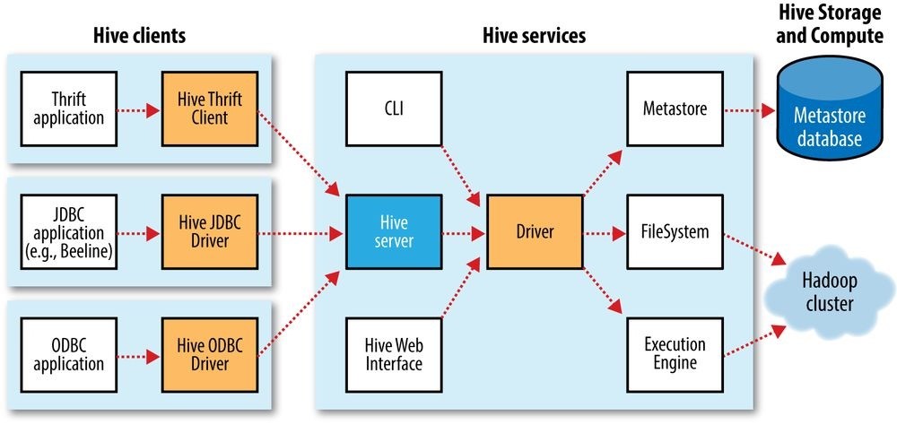
Figure 17-1. Hive architecture
The Metastore
The metastore is the central repository of Hive metadata. The metastore is divided into two pieces: a service and the backing store for the data. By default, the metastore service runs in the same JVM as the Hive service and contains an embedded Derby database instance backed by the local disk. This is called the embedded metastore configuration (see Figure 17-2).
Using an embedded metastore is a simple way to get started with Hive; however, only one embedded Derby database can access the database files on disk at any one time, which means you can have only one Hive session open at a time that accesses the same metastore. Trying to start a second session produces an error when it attempts to open a connection to the metastore.
The solution to supporting multiple sessions (and therefore multiple users) is to use a standalone database. This configuration is referred to as a local metastore, since the metastore service still runs in the same process as the Hive service but connects to a database running in a separate process, either on the same machine or on a remote machine. Any JDBC-compliant database may be used by setting the javax.jdo.option.* configuration properties listed in Table 17-1.108]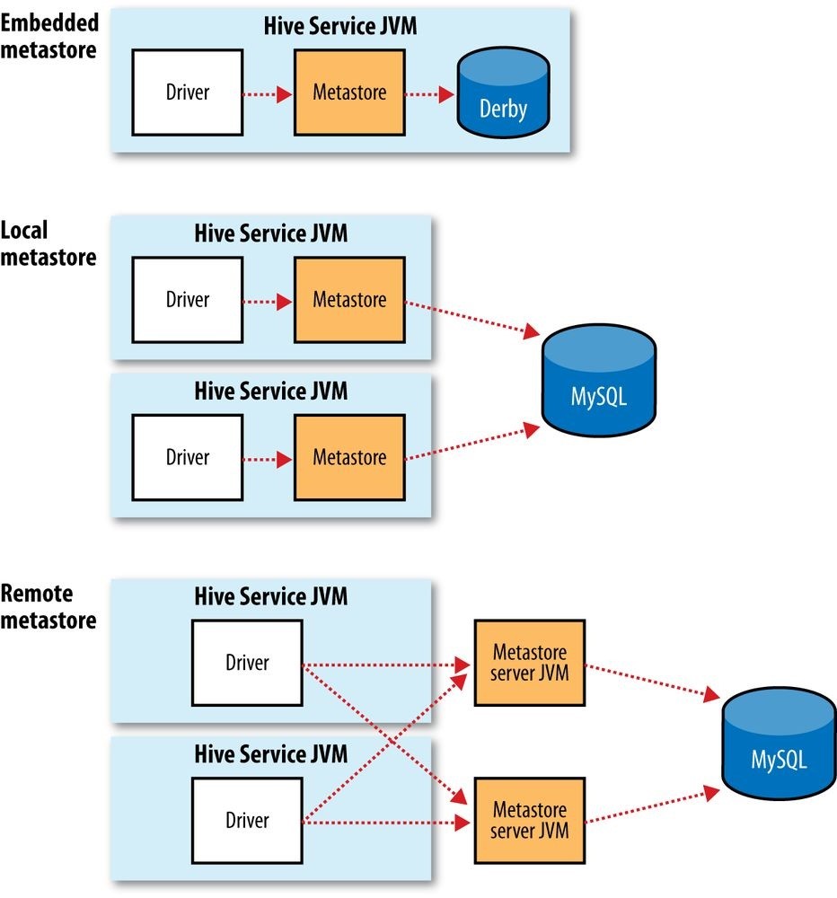
Figure 17-2. Metastore configurations
MySQL is a popular choice for the standalone metastore. In this case, the javax.jdo.option.ConnectionURL property is set to jdbc:mysql://host/dbname? createDatabaseIfNotExist=true, and javax.jdo.option.ConnectionDriverName is set to com.mysql.jdbc.Driver. (The username and password should be set too, of course.) The JDBC driver JAR file for MySQL (Connector/J) must be on Hive’s classpath, which is simply achieved by placing it in Hive’s lib directory.
Going a step further, there’s another metastore configuration called a remote metastore, where one or more metastore servers run in separate processes to the Hive service. This brings better manageability and security because the database tier can be completely firewalled off, and the clients no longer need the database credentials.
A Hive service is configured to use a remote metastore by setting hive.metastore.uris to the metastore server URI(s), separated by commas if there is more than one. Metastore server URIs are of the form thrift://host:port, where the port corresponds to the one set by METASTOREPORT when starting the metastore server (see Hive Services).
_Table 17-1. Important metastore configuration properties
Property name Type Default value Description
hive.metastore . URI /user/hive/ The directory relative to fs.defaultFS where managed warehouse.dir warehouse tables are stored.
| hive.metastore.uris | Comma- Not set separated URIs |
If not set (the default), use an in-process metastore; otherwise, connect to one or more remote metastores, specified by a list of URIs. Clients connect in a roundrobin fashion when there are multiple remote servers. |
|---|---|---|
javax.jdo.option. URI jdbc:derby:;database The JDBC URL of the metastore database.
ConnectionURL Name=metastore_db;
create=true
| javax.jdo.option. String ConnectionDriverName | org.apache.derby. jdbc.EmbeddedDriver | The JDBC driver classname. | |
|---|---|---|---|
| javax.jdo.option. ConnectionUserName |
String | APP | The JDBC username. |
| javax.jdo.option. ConnectionPassword |
String | mine | The JDBC password. |
Comparison with Traditional Databases
Although Hive resembles a traditional database in many ways (such as supporting a SQL interface), its original HDFS and MapReduce underpinnings mean that there are a number of architectural differences that have directly influenced the features that Hive supports. Over time, however, these limitations have been (and continue to be) removed, with the result that Hive looks and feels more like a traditional database with every year that passes.
Schema on Read Versus Schema on Write
In a traditional database, a table’s schema is enforced at data load time. If the data being loaded doesn’t conform to the schema, then it is rejected. This design is sometimes called schema on write because the data is checked against the schema when it is written into the database.
Hive, on the other hand, doesn’t verify the data when it is loaded, but rather when a query is issued. This is called schema on read.
There are trade-offs between the two approaches. Schema on read makes for a very fast initial load, since the data does not have to be read, parsed, and serialized to disk in the database’s internal format. The load operation is just a file copy or move. It is more flexible, too: consider having two schemas for the same underlying data, depending on the analysis being performed. (This is possible in Hive using external tables; see Managed Tables and External Tables.)
Schema on write makes query time performance faster because the database can index columns and perform compression on the data. The trade-off, however, is that it takes longer to load data into the database. Furthermore, there are many scenarios where the schema is not known at load time, so there are no indexes to apply, because the queries have not been formulated yet. These scenarios are where Hive shines.
Updates, Transactions, and Indexes
Updates, transactions, and indexes are mainstays of traditional databases. Yet, until recently, these features have not been considered a part of Hive’s feature set. This is because Hive was built to operate over HDFS data using MapReduce, where full-table scans are the norm and a table update is achieved by transforming the data into a new table. For a data warehousing application that runs over large portions of the dataset, this works well.
Hive has long supported adding new rows in bulk to an existing table by using INSERT INTO to add new data files to a table. From release 0.14.0, finer-grained changes are possible, so you can call INSERT INTO TABLE…VALUES to insert small batches of values computed in SQL. In addition, it is possible to UPDATE and DELETE rows in a table.
HDFS does not provide in-place file updates, so changes resulting from inserts, updates, and deletes are stored in small delta files. Delta files are periodically merged into the base table files by MapReduce jobs that are run in the background by the metastore. These features only work in the context of transactions (introduced in Hive 0.13.0), so the table they are being used on needs to have transactions enabled on it. Queries reading the table are guaranteed to see a consistent snapshot of the table.
Hive also has support for table- and partition-level locking. Locks prevent, for example, one process from dropping a table while another is reading from it. Locks are managed transparently using ZooKeeper, so the user doesn’t have to acquire or release them, although it is possible to get information about which locks are being held via the SHOW LOCKS statement. By default, locks are not enabled.
Hive indexes can speed up queries in certain cases. A query such as SELECT * from t WHERE x = a, for example, can take advantage of an index on column x, since only a small portion of the table’s files need to be scanned. There are currently two index types: compact and bitmap. (The index implementation was designed to be pluggable, so it’s expected that a variety of implementations will emerge for different use cases.)
Compact indexes store the HDFS block numbers of each value, rather than each file offset, so they don’t take up much disk space but are still effective for the case where values are clustered together in nearby rows. Bitmap indexes use compressed bitsets to efficiently store the rows that a particular value appears in, and they are usually appropriate for lowcardinality columns (such as gender or country).
SQL-on-Hadoop Alternatives
In the years since Hive was created, many other SQL-on-Hadoop engines have emerged to address some of Hive’s limitations. Cloudera Impala, an open source interactive SQL engine, was one of the first, giving an order of magnitude performance boost compared to Hive running on MapReduce. Impala uses a dedicated daemon that runs on each datanode in the cluster. When a client runs a query it contacts an arbitrary node running an Impala daemon, which acts as a coordinator node for the query. The coordinator sends work to other Impala daemons in the cluster and combines their results into the full result set for the query. Impala uses the Hive metastore and supports Hive formats and most HiveQL constructs (plus SQL-92), so in practice it is straightforward to migrate between the two systems, or to run both on the same cluster.
Hive has not stood still, though, and since Impala was launched, the “Stinger” initiative by Hortonworks has improved the performance of Hive through support for Tez as an execution engine, and the addition of a vectorized query engine among other improvements.
Other prominent open source Hive alternatives include Presto from Facebook, Apache Drill, and Spark SQL. Presto and Drill have similar architectures to Impala, although Drill targets SQL:2011 rather than HiveQL. Spark SQL uses Spark as its underlying engine, and lets you embed SQL queries in Spark programs.
NOTE
Spark SQL is different to using the Spark execution engine from within Hive (“Hive on Spark,” see Execution engines). Hive, on Spark provides all the features of Hive since it is a part of the Hive project. Spark SQL, on the other hand, is a new SQL engine that offers some level of Hive compatibility.
Apache Phoenix takes a different approach entirely: it provides SQL on HBase. SQL access is through a JDBC driver that turns queries into HBase scans and takes advantage of HBase coprocessors to perform server-side aggregation. Metadata is stored in HBase, too.
HiveQL
Hive’s SQL dialect, called HiveQL, is a mixture of SQL-92, MySQL, and Oracle’s SQL dialect. The level of SQL-92 support has improved over time, and will likely continue to get better. HiveQL also provides features from later SQL standards, such as window functions (also known as analytic functions) from SQL:2003. Some of Hive’s nonstandard extensions to SQL were inspired by MapReduce, such as multitable inserts (see Multitable insert) and the TRANSFORM, MAP, and REDUCE clauses (see MapReduce Scripts).
This chapter does not provide a complete reference to HiveQL; for that, see the Hive documentation. Instead, we focus on commonly used features and pay particular attention to features that diverge from either SQL-92 or popular databases such as MySQL. Table 17-2 provides a high-level comparison of SQL and HiveQL.
Table 17-2. A high-level comparison of SQL and HiveQL
Feature SQL HiveQL References
Updates UPDATE, INSERT, DELETE UPDATE, INSERT, DELETE Inserts; Updates,
| Transactions Supported | Limited support |
|---|---|
Transactions, and
Indexes
Indexes Supported Supported
| Data types | Integral, floating-point, fixed-point, text and binary strings, temporal | Boolean, integral, floating-point, fixedpoint, text and binary strings, temporal, array, map, struct | Data Types |
|---|---|---|---|
| Functions | Hundreds of built-in functions | Hundreds of built-in functions | Operators and Functions |
| Multitable inserts | Not supported | Supported | Multitable insert |
| CREATE TABLE…AS SELECT |
Not valid SQL-92, but found in some databases | Supported | CREATE TABLE…AS SELECT |
| SELECT | SQL-92 | SQL-92. SORT BY for partial ordering, LIMIT to limit number of rows returned |
Querying Data |
| Joins | SQL-92, or variants (join tables in the FROM clause, join condition in the WHERE clause) |
Inner joins, outer joins, semi joins, map joins, cross joins | Joins |
| Subqueries | In any clause (correlated or noncorrelated) | In the FROM, WHERE, or HAVING clauses (uncorrelated subqueries not supported) | Subqueries |
| Views | Updatable (materialized or nonmaterialized) | Read-only (materialized views not supported) | Views |
| Extension points | User-defined functions, stored procedures | User-defined functions, MapReduce scripts User-Defined Functions; MapReduce Scripts |
Data Types
Hive supports both primitive and complex data types. Primitives include numeric, Boolean, string, and timestamp types. The complex data types include arrays, maps, and structs. Hive’s data types are listed in Table 17-3. Note that the literals shown are those used from within HiveQL; they are not the serialized forms used in the table’s storage format (see Storage Formats).
Table 17-3. Hive data types
| Category | Type | Description | Literal examples |
|---|---|---|---|
| Primitive | BOOLEAN | True/false value. | TRUE |
| TINYINT | 1-byte (8-bit) signed integer, from –128 to 127. | 1Y | |
| SMALLINT | 2-byte (16-bit) signed integer, from –32,768 to 32,767. | 1S | |
| INT | 4-byte (32-bit) signed integer, from –2,147,483,648 to 2,147,483,647. | 1 | |
| BIGINT | 8-byte (64-bit) signed integer, from –9,223,372,036,854,775,808 to 9,223,372,036,854,775,807. | 1L | |
| FLOAT | 4-byte (32-bit) single-precision floating-point number. | 1.0 | |
| DOUBLE | 8-byte (64-bit) double-precision floating-point number. | 1.0 | |
| DECIMAL | Arbitrary-precision signed decimal number. | 1.0 | |
| STRING | Unbounded variable-length character string. | ‘a’, “a” | |
| VARCHAR | Variable-length character string. | ‘a’, “a” | |
| CHAR | Fixed-length character string. | ‘a’, “a” | |
| BINARY | Byte array. | Not supported | |
| TIMESTAMP Timestamp with nanosecond precision. | 1325502245000, ‘2012-01- 02 03:04:05.123456789’ |
||
| DATE Date. | ‘2012-01-02’ |
Complex ARRAY An ordered collection of fields. The fields must all be of the array(1, 2) [a] same type.
| MAP | An unordered collection of key-value pairs. Keys must be primitives; values may be any type. For a particular map, the keys must be the same type, and the values must be the same type. | map(‘a’, 1, ‘b’, 2) |
|---|---|---|
| STRUCT | A collection of named fields. The fields may be of different types. | struct(‘a’, 1, 1.0),[b] named_struct(‘col1’, ‘a’, ‘col2’, 1, ‘col3’, 1.0) |
| UNION | A value that may be one of a number of defined data types. The value is tagged with an integer (zero-indexed) representing its data type in the union. | create_union(1, ‘a’, 63) |
[a] The literal forms for arrays, maps, structs, and unions are provided as functions. That is, array, map, struct, and create_union are built-in Hive functions.
[b] The columns are named col1, col2, col3, etc.
Primitive types
Hive’s primitive types correspond roughly to Java’s, although some names are influenced by MySQL’s type names (some of which, in turn, overlap with SQL-92’s). There is a BOOLEAN type for storing true and false values. There are four signed integral types: TINYINT, SMALLINT, INT, and BIGINT, which are equivalent to Java’s byte, short, int, and long primitive types, respectively (they are 1-byte, 2-byte, 4-byte, and 8-byte signed integers).
Hive’s floating-point types, FLOAT and DOUBLE, correspond to Java’s float and double, which are 32-bit and 64-bit floating-point numbers.
The DECIMAL data type is used to represent arbitrary-precision decimals, like Java’s
BigDecimal, and are commonly used for representing currency values. DECIMAL values are stored as unscaled integers. The precision is the number of digits in the unscaled value, and the scale is the number of digits to the right of the decimal point. So, for example, DECIMAL(5,2) stores numbers between −999.99 and 999.99. If the scale is omitted then it defaults to 0, so DECIMAL(5)stores numbers in the range −99,999 to 99,999 (i.e., integers).
If the precision is omitted then it defaults to 10, so DECIMAL is equivalent to
DECIMAL(10,0). The maximum allowed precision is 38, and the scale must be no larger than the precision.
There are three Hive data types for storing text. STRING is a variable-length character string with no declared maximum length. (The theoretical maximum size STRING that may be stored is 2 GB, although in practice it may be inefficient to materialize such large values. Sqoop has large object support; see Importing Large Objects.) VARCHAR types are similar except they are declared with a maximum length between 1 and 65355; for example, VARCHAR(100). CHAR types are fixed-length strings that are padded with trailing spaces if necessary; for example, CHAR(100). Trailing spaces are ignored for the purposes of string comparison of CHAR values.
The BINARY data type is for storing variable-length binary data.
The TIMESTAMP data type stores timestamps with nanosecond precision. Hive comes with UDFs for converting between Hive timestamps, Unix timestamps (seconds since the Unix epoch), and strings, which makes most common date operations tractable. TIMESTAMP does not encapsulate a time zone; however, the to_utc_timestamp and from_utc_timestamp functions make it possible to do time zone conversions.
The DATE data type stores a date with year, month, and day components.
Complex types
Hive has four complex types: ARRAY, MAP, STRUCT, and UNION. ARRAY and MAP are like their namesakes in Java, whereas a STRUCT is a record type that encapsulates a set of named fields. A UNION specifies a choice of data types; values must match exactly one of these types.
Complex types permit an arbitrary level of nesting. Complex type declarations must specify the type of the fields in the collection, using an angled bracket notation, as illustrated in this table definition with three columns (one for each complex type):
CREATE TABLE complex ( c1 ARRAY
If we load the table with one row of data for ARRAY, MAP, STRUCT, and UNION, as shown in the “Literal examples” column in Table 17-3 (we’ll see the file format needed to do this in Storage Formats), the following query demonstrates the field accessor operators for each type:
hive> SELECT c1[0], c2[‘b’], c3.c, c4 FROM complex;
1 2 1.0 {1:63}
Operators and Functions
The usual set of SQL operators is provided by Hive: relational operators (such as x = ‘a’ for testing equality, x IS NULL for testing nullity, and x LIKE ‘a%’ for pattern matching), arithmetic operators (such as x + 1 for addition), and logical operators (such as x OR y for logical OR). The operators match those in MySQL, which deviates from SQL-92 because
|| is logical OR, not string concatenation. Use the concat function for the latter in both MySQL and Hive.
Hive comes with a large number of built-in functions — too many to list here — divided into categories that include mathematical and statistical functions, string functions, date functions (for operating on string representations of dates), conditional functions, aggregate functions, and functions for working with XML (using the xpath function) and JSON.
You can retrieve a list of functions from the Hive shell by typing SHOW FUNCTIONS.109] To get brief usage instructions for a particular function, use the DESCRIBE command:
hive> DESCRIBE FUNCTION length;
length(str | binary) - Returns the length of str or number of bytes in binary data
In the case when there is no built-in function that does what you want, you can write your own; see User-Defined Functions.
Conversions
Primitive types form a hierarchy that dictates the implicit type conversions Hive will perform in function and operator expressions. For example, a TINYINT will be converted to an INT if an expression expects an INT; however, the reverse conversion will not occur, and Hive will return an error unless the CAST operator is used.
The implicit conversion rules can be summarized as follows. Any numeric type can be implicitly converted to a wider type, or to a text type (STRING, VARCHAR, CHAR). All the text types can be implicitly converted to another text type. Perhaps surprisingly, they can also be converted to DOUBLE or DECIMAL. BOOLEAN types cannot be converted to any other type, and they cannot be implicitly converted to any other type in expressions. TIMESTAMP and DATE can be implicitly converted to a text type.
You can perform explicit type conversion using CAST. For example, CAST(‘1’ AS INT) will convert the string ‘1’ to the integer value 1. If the cast fails — as it does in CAST(‘X’ AS INT), for example — the expression returns NULL.
Tables
A Hive table is logically made up of the data being stored and the associated metadata describing the layout of the data in the table. The data typically resides in HDFS, although it may reside in any Hadoop filesystem, including the local filesystem or S3. Hive stores the metadata in a relational database and not in, say, HDFS (see The Metastore).
In this section, we look in more detail at how to create tables, the different physical storage formats that Hive offers, and how to import data into tables.
MULTIPLE DATABASE/SCHEMA SUPPORT
Many relational databases have a facility for multiple namespaces, which allows users and applications to be segregated into different databases or schemas. Hive supports the same facility and provides commands such as
CREATE DATABASE dbname, USE dbname, and DROP DATABASE dbname. You can fully qualify a table by writing dbname.tablename. If no database is specified, tables belong to the default database.
Managed Tables and External Tables
When you create a table in Hive, by default Hive will manage the data, which means that Hive moves the data into its warehouse directory. Alternatively, you may create an external table, which tells Hive to refer to the data that is at an existing location outside the warehouse directory.
The difference between the two table types is seen in the LOAD and DROP semantics. Let’s consider a managed table first.
When you load data into a managed table, it is moved into Hive’s warehouse directory. For example, this:
CREATE TABLE managed_table (dummy STRING);
LOAD DATA INPATH ‘/user/tom/data.txt’ INTO table managed_table; will move the file hdfs://user/tom/data.txt into Hive’s warehouse directory for the managed_table table, which is hdfs://user/hive/warehouse/managed_table.110]
NOTE
The load operation is very fast because it is just a move or rename within a filesystem. However, bear in mind that Hive does not check that the files in the table directory conform to the schema declared for the table, even for managed tables. If there is a mismatch, this will become apparent at query time, often by the query returning NULL for a missing field. You can check that the data is being parsed correctly by issuing a simple SELECT statement to retrieve a few rows directly from the table.
If the table is later dropped, using:
DROP TABLE managed_table; the table, including its metadata and its data, is deleted. It bears repeating that since the initial LOAD performed a move operation, and the DROP performed a delete operation, the data no longer exists anywhere. This is what it means for Hive to manage the data.
An external table behaves differently. You control the creation and deletion of the data. The location of the external data is specified at table creation time:
CREATE EXTERNAL TABLE external_table (dummy STRING)
LOCATION ‘/user/tom/external_table’;
LOAD DATA INPATH ‘/user/tom/data.txt’ INTO TABLE external_table;
With the EXTERNAL keyword, Hive knows that it is not managing the data, so it doesn’t move it to its warehouse directory. Indeed, it doesn’t even check whether the external location exists at the time it is defined. This is a useful feature because it means you can create the data lazily after creating the table.
When you drop an external table, Hive will leave the data untouched and only delete the metadata.
So how do you choose which type of table to use? In most cases, there is not much difference between the two (except of course for the difference in DROP semantics), so it is a just a matter of preference. As a rule of thumb, if you are doing all your processing with Hive, then use managed tables, but if you wish to use Hive and other tools on the same dataset, then use external tables. A common pattern is to use an external table to access an initial dataset stored in HDFS (created by another process), then use a Hive transform to move the data into a managed Hive table. This works the other way around, too; an external table (not necessarily on HDFS) can be used to export data from Hive for other applications to use.111]
Another reason for using external tables is when you wish to associate multiple schemas with the same dataset.
Partitions and Buckets
Hive organizes tables into partitions — a way of dividing a table into coarse-grained parts based on the value of a partition column, such as a date. Using partitions can make it faster to do queries on slices of the data.
Tables or partitions may be subdivided further into buckets to give extra structure to the data that may be used for more efficient queries. For example, bucketing by user ID means we can quickly evaluate a user-based query by running it on a randomized sample of the total set of users.
Partitions
To take an example where partitions are commonly used, imagine logfiles where each record includes a timestamp. If we partition by date, then records for the same date will be stored in the same partition. The advantage to this scheme is that queries that are restricted to a particular date or set of dates can run much more efficiently, because they only need to scan the files in the partitions that the query pertains to. Notice that partitioning doesn’t preclude more wide-ranging queries: it is still feasible to query the entire dataset across many partitions.
A table may be partitioned in multiple dimensions. For example, in addition to partitioning logs by date, we might also subpartition each date partition by country to permit efficient queries by location.
Partitions are defined at table creation time using the PARTITIONED BY clause,112] which takes a list of column definitions. For the hypothetical logfiles example, we might define a table with records comprising a timestamp and the log line itself:
CREATE TABLE logs (ts BIGINT, line STRING)
PARTITIONED BY (dt STRING, country STRING);
When we load data into a partitioned table, the partition values are specified explicitly:
LOAD DATA LOCAL INPATH ‘input/hive/partitions/file1’
INTO TABLE logs
PARTITION (dt=’2001-01-01’, country=’GB’);
At the filesystem level, partitions are simply nested subdirectories of the table directory. After loading a few more files into the logs table, the directory structure might look like this:
/user/hive/warehouse/logs
├── dt=2001-01-01/
│ ├── country=GB/
│ │ ├── file1
│ │ └── file2
│ └── country=US/
│ └── file3
└── dt=2001-01-02/
├── country=GB/ │ └── file4
└── country=US/
├── file5
└── file6
The logs table has two date partitions (2001-01-01 and 2001-01-02, corresponding to subdirectories called dt=2001-01-01 and dt=2001-01-02); and two country subpartitions (GB and US, corresponding to nested subdirectories called country=GB and country=US). The datafiles reside in the leaf directories.
We can ask Hive for the partitions in a table using SHOW PARTITIONS:
hive> SHOW PARTITIONS logs; dt=2001-01-01/country=GB dt=2001-01-01/country=US dt=2001-01-02/country=GB dt=2001-01-02/country=US
One thing to bear in mind is that the column definitions in the PARTITIONED BY clause are full-fledged table columns, called partition columns; however, the datafiles do not contain values for these columns, since they are derived from the directory names.
You can use partition columns in SELECT statements in the usual way. Hive performs input pruning to scan only the relevant partitions. For example:
SELECT ts, dt, line FROM logs
WHERE country=’GB’; will only scan file1, file2, and file4. Notice, too, that the query returns the values of the dt partition column, which Hive reads from the directory names since they are not in the datafiles.
Buckets
There are two reasons why you might want to organize your tables (or partitions) into buckets. The first is to enable more efficient queries. Bucketing imposes extra structure on the table, which Hive can take advantage of when performing certain queries. In particular, a join of two tables that are bucketed on the same columns — which include the join columns — can be efficiently implemented as a map-side join.
The second reason to bucket a table is to make sampling more efficient. When working with large datasets, it is very convenient to try out queries on a fraction of your dataset while you are in the process of developing or refining them. We will see how to do efficient sampling at the end of this section.
First, let’s see how to tell Hive that a table should be bucketed. We use the CLUSTERED BY clause to specify the columns to bucket on and the number of buckets:
CREATE TABLE bucketed_users (id INT, name STRING)
CLUSTERED BY (id) INTO 4 BUCKETS;
Here we are using the user ID to determine the bucket (which Hive does by hashing the value and reducing modulo the number of buckets), so any particular bucket will effectively have a random set of users in it.
In the map-side join case, where the two tables are bucketed in the same way, a mapper processing a bucket of the left table knows that the matching rows in the right table are in its corresponding bucket, so it need only retrieve that bucket (which is a small fraction of all the data stored in the right table) to effect the join. This optimization also works when the number of buckets in the two tables are multiples of each other; they do not have to have exactly the same number of buckets. The HiveQL for joining two bucketed tables is shown in Map joins.
The data within a bucket may additionally be sorted by one or more columns. This allows even more efficient map-side joins, since the join of each bucket becomes an efficient merge sort. The syntax for declaring that a table has sorted buckets is:
CREATE TABLE bucketed_users (id INT, name STRING)
CLUSTERED BY (id) SORTED BY (id ASC) INTO 4 BUCKETS;
How can we make sure the data in our table is bucketed? Although it’s possible to load data generated outside Hive into a bucketed table, it’s often easier to get Hive to do the bucketing, usually from an existing table.
WARNING
Hive does not check that the buckets in the datafiles on disk are consistent with the buckets in the table definition (either in number or on the basis of bucketing columns). If there is a mismatch, you may get an error or undefined behavior at query time. For this reason, it is advisable to get Hive to perform the bucketing.
Take an unbucketed users table:
hive> SELECT * FROM users;
0 Nat
2 Joe
3 Kay
4 Ann
To populate the bucketed table, we need to set the hive.enforce.bucketing property to true so that Hive knows to create the number of buckets declared in the table definition. Then it is just a matter of using the INSERT command:
INSERT OVERWRITE TABLE bucketed_users
SELECT FROM users;
Physically, each bucket is just a file in the table (or partition) directory. The filename is not important, but bucket n is the nth file when arranged in lexicographic order. In fact, buckets correspond to MapReduce output file partitions: a job will produce as many buckets (output files) as reduce tasks. We can see this by looking at the layout of the bucketed_users table we just created. Running this command:
hive> dfs -ls /user/hive/warehouse/bucketed_users;
shows that four files were created, with the following names (the names are generated by Hive):
000000_0
000001_0
000002_0
000003_0
The first bucket contains the users with IDs 0 and 4, since for an INT the hash is the integer itself, and the value is reduced modulo the number of buckets — four, in this case:
[113]
hive> dfs -cat /user/hive/warehouse/bucketed_users/000000_0;
0Nat
4Ann
We can see the same thing by sampling the table using the TABLESAMPLE clause, which restricts the query to a fraction of the buckets in the table rather than the whole table:
hive> **SELECT FROM bucketed_users
> TABLESAMPLE(BUCKET 1 OUT OF 4 ON id);
4 Ann
0 Nat
Bucket numbering is 1-based, so this query retrieves all the users from the first of four buckets. For a large, evenly distributed dataset, approximately one-quarter of the table’s rows would be returned. It’s possible to sample a number of buckets by specifying a different proportion (which need not be an exact multiple of the number of buckets, as sampling is not intended to be a precise operation). For example, this query returns half of the buckets:
hive> SELECT FROM bucketed_users
> TABLESAMPLE(BUCKET 1 OUT OF 2 ON id);
4 Ann
0 Nat
2 Joe
Sampling a bucketed table is very efficient because the query only has to read the buckets that match the TABLESAMPLE clause. Contrast this with sampling a nonbucketed table using the rand() function, where the whole input dataset is scanned, even if only a very small sample is needed:
hive> SELECT FROM users
> TABLESAMPLE(BUCKET 1 OUT OF 4 ON rand()); **2 Joe
Storage Formats
There are two dimensions that govern table storage in Hive: the row format and the file format. The row format dictates how rows, and the fields in a particular row, are stored. In Hive parlance, the row format is defined by a SerDe, a portmanteau word for a SerializerDeserializer.
When acting as a deserializer, which is the case when querying a table, a SerDe will deserialize a row of data from the bytes in the file to objects used internally by Hive to operate on that row of data. When used as a serializer, which is the case when performing an INSERT or CTAS (see Importing Data), the table’s SerDe will serialize Hive’s internal representation of a row of data into the bytes that are written to the output file.
The file format dictates the container format for fields in a row. The simplest format is a plain-text file, but there are row-oriented and column-oriented binary formats available, too.
The default storage format: Delimited text
When you create a table with no ROW FORMAT or STORED AS clauses, the default format is delimited text with one row per line.114]
The default row delimiter is not a tab character, but the Ctrl-A character from the set of ASCII control codes (it has ASCII code 1). The choice of Ctrl-A, sometimes written as ^A in documentation, came about because it is less likely to be a part of the field text than a tab character. There is no means for escaping delimiter characters in Hive, so it is important to choose ones that don’t occur in data fields.
The default collection item delimiter is a Ctrl-B character, used to delimit items in an
ARRAY or STRUCT, or in key-value pairs in a MAP. The default map key delimiter is a Ctrl-C character, used to delimit the key and value in a MAP. Rows in a table are delimited by a newline character.
WARNING
The preceding description of delimiters is correct for the usual case of flat data structures, where the complex types contain only primitive types. For nested types, however, this isn’t the whole story, and in fact the level of the nesting determines the delimiter.
For an array of arrays, for example, the delimiters for the outer array are Ctrl-B characters, as expected, but for the inner array they are Ctrl-C characters, the next delimiter in the list. If you are unsure which delimiters Hive uses for a particular nested structure, you can run a command like:
CREATE TABLE nested
AS
SELECT array(array(1, 2), array(3, 4)) FROM dummy; and then use hexdump or something similar to examine the delimiters in the output file.
Hive actually supports eight levels of delimiters, corresponding to ASCII codes 1, 2, … 8, but you can override only the first three.
Thus, the statement:
CREATE TABLE …; is identical to the more explicit:
CREATE TABLE …
ROW FORMAT DELIMITED
FIELDS TERMINATED BY ‘\001’
COLLECTION ITEMS TERMINATED BY ‘\002’
MAP KEYS TERMINATED BY ‘\003’
LINES TERMINATED BY ‘\n’
STORED AS TEXTFILE;
Notice that the octal form of the delimiter characters can be used — 001 for Ctrl-A, for instance.
Internally, Hive uses a SerDe called LazySimpleSerDe for this delimited format, along with the line-oriented MapReduce text input and output formats we saw in Chapter 8. The “lazy” prefix comes about because it deserializes fields lazily — only as they are accessed. However, it is not a compact format because fields are stored in a verbose textual format, so a Boolean value, for instance, is written as the literal string true or false.
The simplicity of the format has a lot going for it, such as making it easy to process with other tools, including MapReduce programs or Streaming, but there are more compact and performant binary storage formats that you might consider using. These are discussed next.
Binary storage formats: Sequence files, Avro datafiles, Parquet files, RCFiles, and ORCFiles
Using a binary format is as simple as changing the STORED AS clause in the CREATE TABLE statement. In this case, the ROW FORMAT is not specified, since the format is controlled by the underlying binary file format.
Binary formats can be divided into two categories: row-oriented formats and columnoriented formats. Generally speaking, column-oriented formats work well when queries access only a small number of columns in the table, whereas row-oriented formats are appropriate when a large number of columns of a single row are needed for processing at the same time.
The two row-oriented formats supported natively in Hive are Avro datafiles (see Chapter 12) and sequence files (see SequenceFile). Both are general-purpose, splittable, compressible formats; in addition, Avro supports schema evolution and multiple language bindings. From Hive 0.14.0, a table can be stored in Avro format using:
SET hive.exec.compress.output=true;
SET avro.output.codec=snappy;
CREATE TABLE … STORED AS AVRO;
Notice that compression is enabled on the table by setting the relevant properties.
Similarly, the declaration STORED AS SEQUENCEFILE can be used to store sequence files in Hive. The properties for compression are listed in Using Compression in MapReduce.
Hive has native support for the Parquet (see Chapter 13), RCFile, and ORCFile columnoriented binary formats (see Other File Formats and Column-Oriented Formats). Here is an example of creating a copy of a table in Parquet format using CREATE TABLE…AS SELECT (see CREATE TABLE…AS SELECT):
CREATE TABLE users_parquet STORED AS PARQUET
AS
SELECT * FROM users;
Using a custom SerDe: RegexSerDe
Let’s see how to use a custom SerDe for loading data. We’ll use a contrib SerDe that uses a regular expression for reading the fixed-width station metadata from a text file:
CREATE TABLE stations (usaf STRING, wban STRING, name STRING) ROW FORMAT SERDE ‘org.apache.hadoop.hive.contrib.serde2.RegexSerDe’ WITH SERDEPROPERTIES (
“input.regex” = “(\d{6}) (\d{5}) (.{29}) .“ );
In previous examples, we have used the DELIMITED keyword to refer to delimited text in the ROW FORMAT clause. In this example, we instead specify a SerDe with the SERDE keyword and the fully qualified classname of the Java class that implements the SerDe, org.apache.hadoop.hive.contrib.serde2.RegexSerDe.
SerDes can be configured with extra properties using the WITH SERDEPROPERTIES clause.
Here we set the input.regex property, which is specific to RegexSerDe.
input.regex is the regular expression pattern to be used during deserialization to turn the line of text forming the row into a set of columns. Java regular expression syntax is used for the matching, and columns are formed from capturing groups of parentheses.115] In this example, there are three capturing groups for usaf (a six-digit identifier), wban (a fivedigit identifier), and name (a fixed-width column of 29 characters).
To populate the table, we use a LOAD DATA statement as before:
LOAD DATA LOCAL INPATH “input/ncdc/metadata/stations-fixed-width.txt” INTO TABLE stations;
Recall that LOAD DATA copies or moves the files to Hive’s warehouse directory (in this case, it’s a copy because the source is the local filesystem). The table’s SerDe is not used for the load operation.
When we retrieve data from the table the SerDe is invoked for deserialization, as we can see from this simple query, which correctly parses the fields for each row:
hive> **SELECT FROM stations LIMIT 4;**
010000 99999 BOGUS NORWAY
010003 99999 BOGUS NORWAY
010010 99999 JAN MAYEN
010013 99999 ROST
As this example demonstrates, RegexSerDe can be useful for getting data into Hive, but due to its inefficiency it should not be used for general-purpose storage. Consider copying the data into a binary storage format instead.
Storage handlers
Storage handlers are used for storage systems that Hive cannot access natively, such as
HBase. Storage handlers are specified using a STORED BY clause, instead of the ROW FORMAT and STORED AS clauses. For more information on HBase integration, see the Hive wiki.
Importing Data
We’ve already seen how to use the LOAD DATA operation to import data into a Hive table (or partition) by copying or moving files to the table’s directory. You can also populate a table with data from another Hive table using an INSERT statement, or at creation time using the CTAS construct, which is an abbreviation used to refer to CREATE TABLE…AS SELECT.
If you want to import data from a relational database directly into Hive, have a look at Sqoop; this is covered in Imported Data and Hive.
Inserts
Here’s an example of an INSERT statement:
INSERT OVERWRITE TABLE target
SELECT col1, col2
FROM source;
For partitioned tables, you can specify the partition to insert into by supplying a PARTITION clause:
INSERT OVERWRITE TABLE target
PARTITION (dt=’2001-01-01’) SELECT col1, col2
FROM source;
The OVERWRITE keyword means that the contents of the target table (for the first example) or the 2001-01-01 partition (for the second example) are replaced by the results of the SELECT statement. If you want to add records to an already populated nonpartitioned table or partition, use INSERT INTO TABLE.
You can specify the partition dynamically by determining the partition value from the SELECT statement:
INSERT OVERWRITE TABLE target
PARTITION (dt)
SELECT col1, col2, dt FROM source;
This is known as a dynamic partition insert.
Multitable insert
In HiveQL, you can turn the INSERT statement around and start with the FROM clause for the same effect:
FROM source
INSERT OVERWRITE TABLE target
SELECT col1, col2;
The reason for this syntax becomes clear when you see that it’s possible to have multiple INSERT clauses in the same query. This so-called multitable insert is more efficient than multiple INSERT statements because the source table needs to be scanned only once to produce the multiple disjoint outputs.
Here’s an example that computes various statistics over the weather dataset:
FROM records2
INSERT OVERWRITE TABLE stations_by_year
SELECT year, COUNT(DISTINCT station) GROUP BY year
INSERT OVERWRITE TABLE records_by_year
SELECT year, COUNT(1)
GROUP BY year
INSERT OVERWRITE TABLE good_records_by_year
SELECT year, COUNT(1)
WHERE temperature != 9999 AND quality IN (0, 1, 4, 5, 9) GROUP BY year;
There is a single source table (records2), but three tables to hold the results from three different queries over the source.
CREATE TABLE…AS SELECT
It’s often very convenient to store the output of a Hive query in a new table, perhaps because it is too large to be dumped to the console or because there are further processing steps to carry out on the result.
The new table’s column definitions are derived from the columns retrieved by the SELECT clause. In the following query, the target table has two columns named col1 and col2 whose types are the same as the ones in the source table:
CREATE TABLE target
AS
SELECT col1, col2
FROM source;
A CTAS operation is atomic, so if the SELECT query fails for some reason, the table is not created.
Altering Tables
Because Hive uses the schema-on-read approach, it’s flexible in permitting a table’s definition to change after the table has been created. The general caveat, however, is that in many cases, it is up to you to ensure that the data is changed to reflect the new structure.
You can rename a table using the ALTER TABLE statement:
ALTER TABLE source RENAME TO target;
In addition to updating the table metadata, ALTER TABLE moves the underlying table directory so that it reflects the new name. In the current example,
/user/hive/warehouse/source is renamed to /user/hive/warehouse/target. (An external table’s underlying directory is not moved; only the metadata is updated.)
Hive allows you to change the definition for columns, add new columns, or even replace all existing columns in a table with a new set.
For example, consider adding a new column:
ALTER TABLE target ADD COLUMNS (col3 STRING);
The new column col3 is added after the existing (nonpartition) columns. The datafiles are not updated, so queries will return null for all values of col3 (unless of course there were extra fields already present in the files). Because Hive does not permit updating existing records, you will need to arrange for the underlying files to be updated by another mechanism. For this reason, it is more common to create a new table that defines new columns and populates them using a SELECT statement.
Changing a column’s metadata, such as a column’s name or data type, is more straightforward, assuming that the old data type can be interpreted as the new data type.
To learn more about how to alter a table’s structure, including adding and dropping partitions, changing and replacing columns, and changing table and SerDe properties, see the Hive wiki.
Dropping Tables
The DROP TABLE statement deletes the data and metadata for a table. In the case of external tables, only the metadata is deleted; the data is left untouched.
If you want to delete all the data in a table but keep the table definition, use TRUNCATE TABLE. For example:
TRUNCATE TABLE my_table;
This doesn’t work for external tables; instead, use dfs -rmr (from the Hive shell) to remove the external table directory directly.
In a similar vein, if you want to create a new, empty table with the same schema as another table, then use the LIKE keyword:
CREATE TABLE new_table LIKE existing_table;
Querying Data
This section discusses how to use various forms of the SELECT statement to retrieve data from Hive.
Sorting and Aggregating
Sorting data in Hive can be achieved by using a standard ORDER BY clause. ORDER BY performs a parallel total sort of the input (like that described in Total Sort). When a globally sorted result is not required — and in many cases it isn’t — you can use Hive’s nonstandard extension, SORT BY, instead. SORT BY produces a sorted file per reducer.
In some cases, you want to control which reducer a particular row goes to — typically so you can perform some subsequent aggregation. This is what Hive’s DISTRIBUTE BY clause does. Here’s an example to sort the weather dataset by year and temperature, in such a way as to ensure that all the rows for a given year end up in the same reducer partition:116]
hive> FROM records2
> SELECT year, temperature
> DISTRIBUTE BY year
> SORT BY year ASC, temperature DESC;
1949 111
1949 78
1950 22
1950 0
1950 -11
A follow-on query (or a query that nests this query as a subquery; see Subqueries) would be able to use the fact that each year’s temperatures were grouped and sorted (in descending order) in the same file.
If the columns for SORT BY and DISTRIBUTE BY are the same, you can use CLUSTER BY as a shorthand for specifying both.
MapReduce Scripts
Using an approach like Hadoop Streaming, the TRANSFORM, MAP, and REDUCE clauses make it possible to invoke an external script or program from Hive. Suppose we want to use a script to filter out rows that don’t meet some condition, such as the script in Example 17-1, which removes poor-quality readings.
Example 17-1. Python script to filter out poor-quality weather records
#!/usr/bin/env python
import re import sys
for line in sys.stdin:
(year, temp, q) = line.strip().split() if (temp != “9999” and re.match(“[01459]”, q)): print “%s\t%s” % (year, temp)
We can use the script as follows:
hive> ADD FILE /Users/tom/book-workspace/hadoop-book/ch17-hive/ src/main/python/is_good_quality.py; hive> FROM records2
> SELECT TRANSFORM(year, temperature, quality)
> USING ‘is_good_quality.py’
> AS year, temperature;
1950 0
1950 22
1950 -11
1949 111
1949 78
Before running the query, we need to register the script with Hive. This is so Hive knows to ship the file to the Hadoop cluster (see Distributed Cache).
The query itself streams the year, temperature, and quality fields as a tab-separated line to the is_good_quality.py script, and parses the tab-separated output into year and temperature fields to form the output of the query.
This example has no reducers. If we use a nested form for the query, we can specify a map and a reduce function. This time we use the MAP and REDUCE keywords, but SELECT TRANSFORM in both cases would have the same result. (Example 2-10 includes the source for the max_temperature_reduce.py script):
FROM (
FROM records2
MAP year, temperature, quality
USING ‘is_good_quality.py’
AS year, temperature) map_output
REDUCE year, temperature
USING ‘max_temperature_reduce.py’
AS year, temperature;
Joins
One of the nice things about using Hive, rather than raw MapReduce, is that Hive makes performing commonly used operations very simple. Join operations are a case in point, given how involved they are to implement in MapReduce (see Joins).
Inner joins
The simplest kind of join is the inner join, where each match in the input tables results in a row in the output. Consider two small demonstration tables, sales (which lists the names of people and the IDs of the items they bought) and things (which lists the item IDs and their names):
hive> SELECT * FROM sales;
Joe 2
Hank 4
Ali 0
Eve 3 Hank 2 hive> SELECT * FROM things;
2 Tie
4 Coat
3 Hat
1 Scarf
We can perform an inner join on the two tables as follows:
hive> SELECT sales., things.
> FROM sales JOIN things ON (sales.id = things.id);
Joe 2 2 Tie
Hank 4 4 Coat
Eve 3 3 Hat
Hank 2 2 Tie
The table in the FROM clause (sales) is joined with the table in the JOIN clause (things), using the predicate in the ON clause. Hive only supports equijoins, which means that only equality can be used in the join predicate, which here matches on the id column in both tables.
In Hive, you can join on multiple columns in the join predicate by specifying a series of expressions, separated by AND keywords. You can also join more than two tables by supplying additional JOIN…ON… clauses in the query. Hive is intelligent about trying to
performed in less than one MapReduce job per join if the same column is used in the join condition.117] You can see how many MapReduce jobs Hive will use for any particular query by prefixing it with the EXPLAIN keyword:
EXPLAIN
SELECT sales., things.
FROM sales JOIN things ON (sales.id = things.id);
The EXPLAIN output includes many details about the execution plan for the query, including the abstract syntax tree, the dependency graph for the stages that Hive will execute, and information about each stage. Stages may be MapReduce jobs or operations such as file moves. For even more detail, prefix the query with EXPLAIN EXTENDED.
Hive currently uses a rule-based query optimizer for determining how to execute a query, but a cost-based optimizer is available from Hive 0.14.0.
Outer joins
Outer joins allow you to find nonmatches in the tables being joined. In the current example, when we performed an inner join, the row for Ali did not appear in the output, because the ID of the item she purchased was not present in the things table. If we change the join type to LEFT OUTER JOIN, the query will return a row for every row in the left table (sales), even if there is no corresponding row in the table it is being joined to (things):
hive> SELECT sales., things.
> FROM sales LEFT OUTER JOIN things ON (sales.id = things.id); Joe 2 2 Tie
Hank 4 4 Coat
Ali 0 NULL NULL
Eve 3 3 Hat
Hank 2 2 Tie
Notice that the row for Ali is now returned, and the columns from the things table are NULL because there is no match.
Hive also supports right outer joins, which reverses the roles of the tables relative to the left join. In this case, all items from the things table are included, even those that weren’t purchased by anyone (a scarf):
hive> SELECT sales., things.
> FROM sales RIGHT OUTER JOIN things ON (sales.id = things.id);
Joe 2 2 Tie
Hank 2 2 Tie
Hank 4 4 Coat
Eve 3 3 Hat
NULL NULL 1 Scarf
Finally, there is a full outer join, where the output has a row for each row from both tables in the join:
hive> SELECT sales., things.
> FROM sales FULL OUTER JOIN things ON (sales.id = things.id);
Ali 0 NULL NULL
NULL NULL 1 Scarf
Hank 2 2 Tie
Joe 2 2 Tie
Eve 3 3 Hat
Hank 4 4 Coat
Semi joins
Consider this IN subquery, which finds all the items in the things table that are in the sales table:
SELECT
FROM things
WHERE things.id IN (SELECT id from sales); We can also express it as follows:
hive> SELECT
> FROM things LEFT SEMI JOIN sales ON (sales.id = things.id);
2 Tie
4 Coat 3 Hat
There is a restriction that we must observe for LEFT SEMI JOIN queries: the right table (sales) may appear only in the ON clause. It cannot be referenced in a SELECT expression, for example.
Map joins
Consider the original inner join again:
SELECT sales., things.
FROM sales JOIN things ON (sales.id = things.id);
If one table is small enough to fit in memory, as things is here, Hive can load it into memory to perform the join in each of the mappers. This is called a map join.
The job to execute this query has no reducers, so this query would not work for a RIGHT or FULL OUTER JOIN, since absence of matching can be detected only in an aggregating (reduce) step across all the inputs.
Map joins can take advantage of bucketed tables (see Buckets), since a mapper working on a bucket of the left table needs to load only the corresponding buckets of the right table to perform the join. The syntax for the join is the same as for the in-memory case shown earlier; however, you also need to enable the optimization with the following:
SET hive.optimize.bucketmapjoin=true;
Subqueries
A subquery is a SELECT statement that is embedded in another SQL statement. Hive has limited support for subqueries, permitting a subquery in the FROM clause of a SELECT statement, or in the WHERE clause in certain cases.
station:
SELECT station, year, AVG(max_temperature)
FROM (
SELECT station, year, MAX(temperature) AS max_temperature FROM records2
WHERE temperature != 9999 AND quality IN (0, 1, 4, 5, 9)
GROUP BY station, year
) mt
GROUP BY station, year;
The FROM subquery is used to find the maximum temperature for each station/date combination, and then the outer query uses the AVG aggregate function to find the average of the maximum temperature readings for each station/date combination.
The outer query accesses the results of the subquery like it does a table, which is why the subquery must be given an alias (mt). The columns of the subquery have to be given unique names so that the outer query can refer to them.
Views
A view is a sort of “virtual table” that is defined by a SELECT statement. Views can be used to present data to users in a way that differs from the way it is actually stored on disk. Often, the data from existing tables is simplified or aggregated in a particular way that makes it convenient for further processing. Views may also be used to restrict users’ access to particular subsets of tables that they are authorized to see.
In Hive, a view is not materialized to disk when it is created; rather, the view’s SELECT statement is executed when the statement that refers to the view is run. If a view performs extensive transformations on the base tables or is used frequently, you may choose to manually materialize it by creating a new table that stores the contents of the view (see
CREATE TABLE…AS SELECT).
We can use views to rework the query from the previous section for finding the mean maximum temperature for every year and weather station. First, let’s create a view for valid records — that is, records that have a particular quality value:
CREATE VIEW validrecords
AS
SELECT *
FROM records2
WHERE temperature != 9999 AND quality IN (0, 1, 4, 5, 9);
When we create a view, the query is not run; it is simply stored in the metastore. Views are included in the output of the SHOW TABLES command, and you can see more details about a particular view, including the query used to define it, by issuing the DESCRIBE EXTENDED _view_name command.
Next, let’s create a second view of maximum temperatures for each station and year. It is based on the valid_records view:
CREATE VIEW max_temperatures (station, year, max_temperature) AS
SELECT station, year, MAX(temperature)
FROM valid_records
GROUP BY station, year;
In this view definition, we list the column names explicitly. We do this because the maximum temperature column is an aggregate expression, and otherwise Hive would create a column alias for us (such as _c2). We could equally well have used an AS clause in the SELECT to name the column.
With the views in place, we can now use them by running a query:
SELECT station, year, AVG(max_temperature)
FROM max_temperatures
GROUP BY station, year;
The result of the query is the same as that of running the one that uses a subquery. In particular, Hive creates the same number of MapReduce jobs for both: two in each case, one for each GROUP BY. This example shows that Hive can combine a query on a view into a sequence of jobs that is equivalent to writing the query without using a view. In other words, Hive won’t needlessly materialize a view, even at execution time.
Views in Hive are read-only, so there is no way to load or insert data into an underlying base table via a view.
User-Defined Functions
Sometimes the query you want to write can’t be expressed easily (or at all) using the builtin functions that Hive provides. By allowing you to write a user-defined function (UDF),
Hive makes it easy to plug in your own processing code and invoke it from a Hive query.
UDFs have to be written in Java, the language that Hive itself is written in. For other languages, consider using a SELECT TRANSFORM query, which allows you to stream data through a user-defined script (MapReduce Scripts).
There are three types of UDF in Hive: (regular) UDFs, user-defined aggregate functions (UDAFs), and user-defined table-generating functions (UDTFs). They differ in the number of rows that they accept as input and produce as output:
A UDF operates on a single row and produces a single row as its output. Most functions, such as mathematical functions and string functions, are of this type. A UDAF works on multiple input rows and creates a single output row. Aggregate functions include such functions as COUNT and MAX.
A UDTF operates on a single row and produces multiple rows — a table — as output.
Table-generating functions are less well known than the other two types, so let’s look at an example. Consider a table with a single column, x, which contains arrays of strings. It’s instructive to take a slight detour to see how the table is defined and populated:
CREATE TABLE arrays (x ARRAY
ROW FORMAT DELIMITED
FIELDS TERMINATED BY ‘\001’
COLLECTION ITEMS TERMINATED BY ‘\002’;
Notice that the ROW FORMAT clause specifies that the entries in the array are delimited by Ctrl-B characters. The example file that we are going to load has the following contents, where ^B is a representation of the Ctrl-B character to make it suitable for printing:
a^Bb c^Bd^Be
After running a LOAD DATA command, the following query confirms that the data was loaded correctly:
hive> SELECT * FROM arrays;
[“a”,”b”]
[“c”,”d”,”e”]
Next, we can use the explode UDTF to transform this table. This function emits a row for each entry in the array, so in this case the type of the output column y is STRING. The result is that the table is flattened into five rows:
hive> SELECT explode(x) AS y FROM arrays; a b c d e
SELECT statements using UDTFs have some restrictions (e.g., they cannot retrieve additional column expressions), which make them less useful in practice. For this reason, Hive supports LATERAL VIEW queries, which are more powerful. LATERAL VIEW queries are not covered here, but you may find out more about them in the Hive wiki.
Writing a UDF
To illustrate the process of writing and using a UDF, we’ll write a simple UDF to trim characters from the ends of strings. Hive already has a built-in function called trim, so we’ll call ours strip. The code for the Strip Java class is shown in Example 17-2. Example 17-2. A UDF for stripping characters from the ends of strings
package com.hadoopbook.hive;
import org.apache.commons.lang.StringUtils; import org.apache.hadoop.hive.ql.exec.UDF; import org.apache.hadoop.io.Text;
public class Strip extends UDF { private Text result = new Text();
public Text evaluate(Text str) { if (str == null) { return null;
}
result.set(StringUtils.strip(str.toString())); return result;
} public Text evaluate(Text str, String stripChars) { if (str == null) { return null;
}
result.set(StringUtils.strip(str.toString(), stripChars)); return result;
} }
A UDF must satisfy the following two properties:
A UDF must be a subclass of org.apache.hadoop.hive.ql.exec.UDF. A UDF must implement at least one evaluate() method.
The evaluate() method is not defined by an interface, since it may take an arbitrary number of arguments, of arbitrary types, and it may return a value of arbitrary type. Hive introspects the UDF to find the evaluate() method that matches the Hive function that was invoked.
The Strip class has two evaluate() methods. The first strips leading and trailing whitespace from the input, and the second can strip any of a set of supplied characters from the ends of the string. The actual string processing is delegated to the StringUtils class from the Apache Commons project, which makes the only noteworthy part of the code the use of Text from the Hadoop Writable library. Hive actually supports Java primitives in UDFs (and a few other types, such as java.util.List and java.util.Map), so a signature like: public String evaluate(String str)
would work equally well. However, by using Text we can take advantage of object reuse, which can bring efficiency savings, so this is preferred in general.
To use the UDF in Hive, we first need to package the compiled Java class in a JAR file. You can do this by typing mvn package with the book’s example code. Next, we register the function in the metastore and give it a name using the CREATE FUNCTION statement:
CREATE FUNCTION strip AS ‘com.hadoopbook.hive.Strip’
USING JAR ‘/path/to/hive-examples.jar’;
When using Hive locally, a local file path is sufficient, but on a cluster you should copy the JAR file into HDFS and use an HDFS URI in the USING JAR clause.
The UDF is now ready to be used, just like a built-in function:
hive> SELECT strip(‘ bee ‘) FROM dummy; bee
hive> SELECT strip(‘banana’, ‘ab’) FROM dummy; nan
Notice that the UDF’s name is not case sensitive:
hive> SELECT STRIP(‘ bee ‘) FROM dummy; bee
If you want to remove the function, use the DROP FUNCTION statement:
DROP FUNCTION strip;
It’s also possible to create a function for the duration of the Hive session, so it is not persisted in the metastore, using the TEMPORARY keyword:
ADD JAR /path/to/hive-examples.jar;
CREATE TEMPORARY FUNCTION strip AS ‘com.hadoopbook.hive.Strip’;
When using temporary functions, it may be useful to create a .hiverc file in your home directory containing the commands to define your UDFs. The file will be automatically run at the beginning of each Hive session.
NOTE
As an alternative to calling ADD JAR at launch time, you can specify a path where Hive looks for auxiliary JAR files to put on its classpath (including the task classpath). This technique is useful for automatically adding your own library of UDFs every time you run Hive.
There are two ways of specifying the path. Either pass the —auxpath option to the hive command:
% hive —auxpath /path/to/hive-examples.jar or set the HIVE_AUX_JARS_PATH environment variable before invoking Hive. The auxiliary path may be a commaseparated list of JAR file paths or a directory containing JAR files.
Writing a UDAF
An aggregate function is more difficult to write than a regular UDF. Values are aggregated in chunks (potentially across many tasks), so the implementation has to be capable of combining partial aggregations into a final result. The code to achieve this is best explained by example, so let’s look at the implementation of a simple UDAF for calculating the maximum of a collection of integers (Example 17-3).
Example 17-3. A UDAF for calculating the maximum of a collection of integers
package com.hadoopbook.hive;
import org.apache.hadoop.hive.ql.exec.UDAF; import org.apache.hadoop.hive.ql.exec.UDAFEvaluator; import org.apache.hadoop.io.IntWritable; public class Maximum extends UDAF {
public static class MaximumIntUDAFEvaluator implements UDAFEvaluator {
private IntWritable result;
public void init() { result = null;
} public boolean iterate(IntWritable value) { if (value == null) { return true;
}
if (result == null) { result = new IntWritable(value.get());
} else {
result.set(Math.max(result.get(), value.get()));
}
return true;
}
public IntWritable terminatePartial() { return result;
}
public boolean merge(IntWritable other) { return iterate(other);
}
public IntWritable terminate() { return result;
}
} }
The class structure is slightly different from the one for UDFs. A UDAF must be a subclass of org.apache.hadoop.hive.ql.exec.UDAF (note the “A” in UDAF) and contain one or more nested static classes implementing org.apache.hadoop.hive.ql.exec.UDAFEvaluator. In this example, there is a single nested class, MaximumIntUDAFEvaluator, but we could add more evaluators, such as MaximumLongUDAFEvaluator, MaximumFloatUDAFEvaluator, and so on, to provide overloaded forms of the UDAF for finding the maximum of a collection of longs, floats, and so on.
An evaluator must implement five methods, described in turn here (the flow is illustrated in Figure 17-3): init()
The init() method initializes the evaluator and resets its internal state. In
MaximumIntUDAFEvaluator, we set the IntWritable object holding the final result to null. We use null to indicate that no values have been aggregated yet, which has the desirable effect of making the maximum value of an empty set NULL. iterate()
The iterate() method is called every time there is a new value to be aggregated. The evaluator should update its internal state with the result of performing the aggregation. The arguments that iterate() takes correspond to those in the Hive function from which it was called. In this example, there is only one argument. The value is first checked to see whether it is null, and if it is, it is ignored. Otherwise, the result instance variable is set either to value’s integer value (if this is the first value that has been seen) or to the larger of the current result and value (if one or more values have already been seen). We return true to indicate that the input value was valid. terminatePartial()
The terminatePartial() method is called when Hive wants a result for the partial aggregation. The method must return an object that encapsulates the state of the aggregation. In this case, an IntWritable suffices because it encapsulates either the maximum value seen or null if no values have been processed.
merge()
The merge() method is called when Hive decides to combine one partial aggregation with another. The method takes a single object, whose type must correspond to the return type of the terminatePartial() method. In this example, the merge() method can simply delegate to the iterate() method because the partial aggregation is represented in the same way as a value being aggregated. This is not generally the case (we’ll see a more general example later), and the method should implement the logic to combine the evaluator’s state with the state of the partial aggregation. terminate()
The terminate() method is called when the final result of the aggregation is needed. The evaluator should return its state as a value. In this case, we return the result instance variable.
Let’s exercise our new function:
hive> CREATE TEMPORARY FUNCTION maximum AS ‘com.hadoopbook.hive.Maximum’; hive> SELECT maximum(temperature) FROM records; 111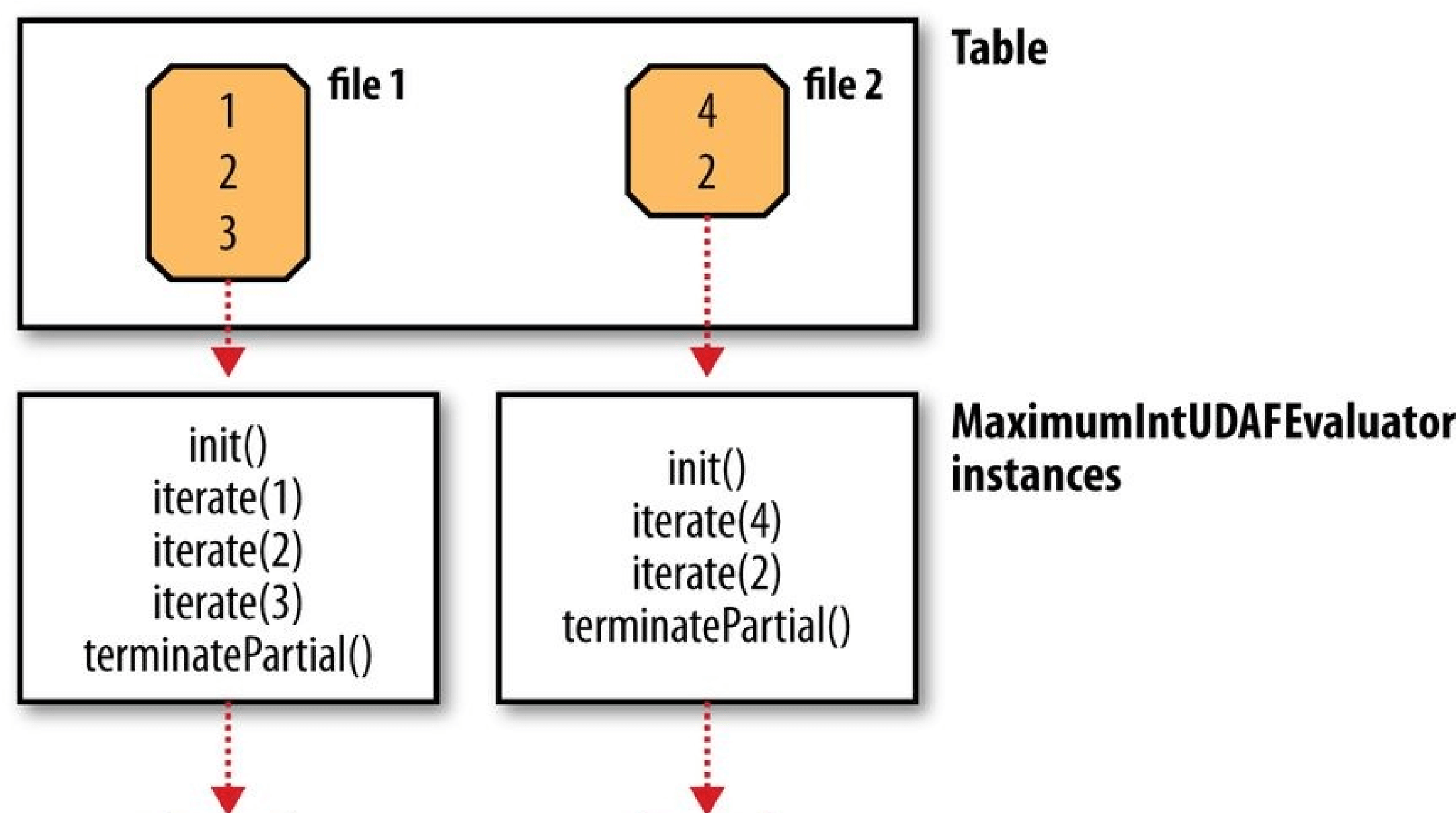
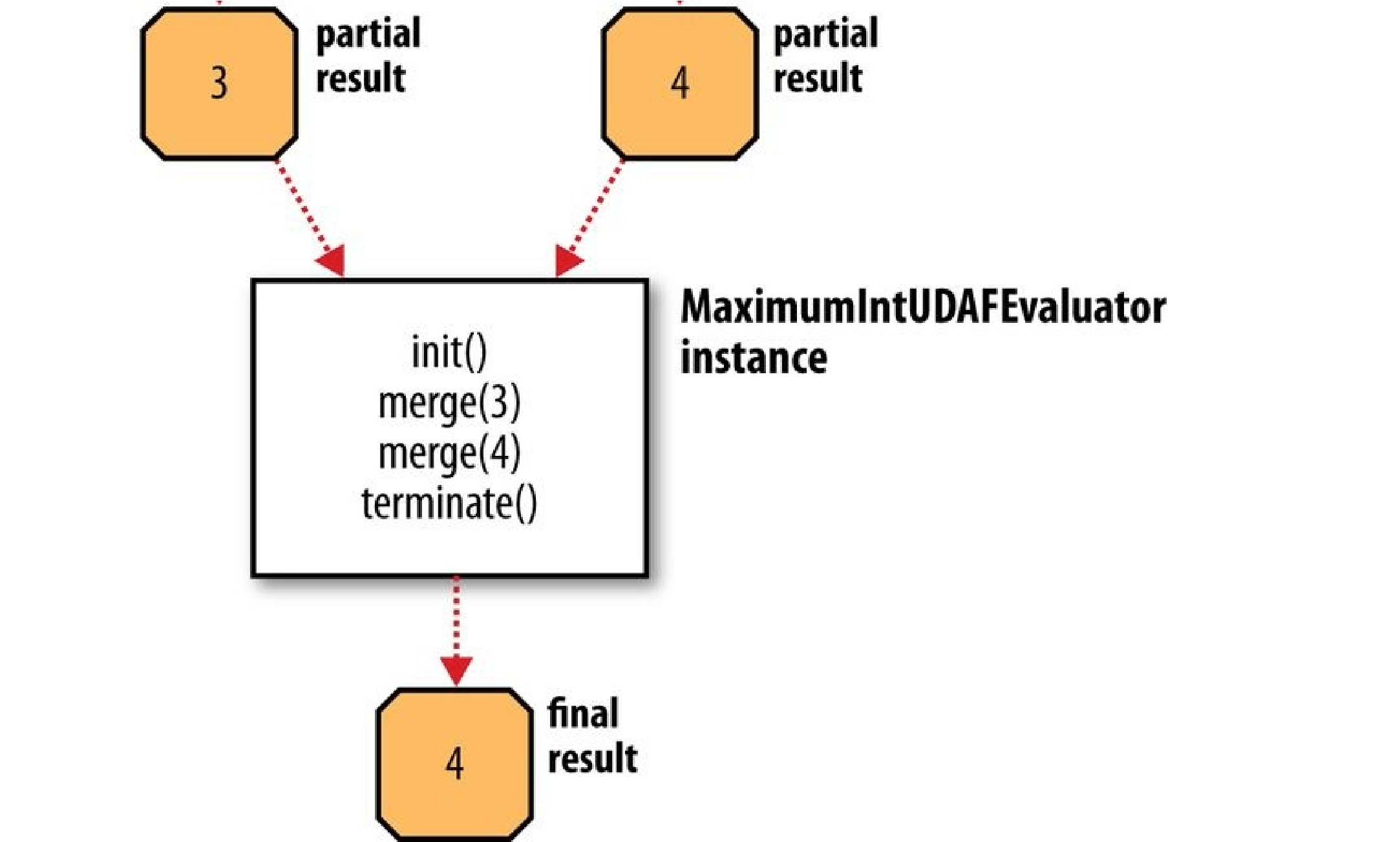
Figure 17-3. Data flow with partial results for a UDAF
A more complex UDAF
The previous example is unusual in that a partial aggregation can be represented using the same type (IntWritable) as the final result. This is not generally the case for more complex aggregate functions, as can be seen by considering a UDAF for calculating the mean (average) of a collection of double values. It’s not mathematically possible to combine partial means into a final mean value (see Combiner Functions). Instead, we can represent the partial aggregation as a pair of numbers: the cumulative sum of the double values processed so far, and the number of values.
This idea is implemented in the UDAF shown in Example 17-4. Notice that the partial aggregation is implemented as a “struct” nested static class, called PartialResult, which Hive is intelligent enough to serialize and deserialize, since we are using field types that Hive can handle (Java primitives in this case).
In this example, the merge() method is different from iterate() because it combines the partial sums and partial counts by pairwise addition. In addition to this, the return type of terminatePartial() is PartialResult — which, of course, is never seen by the user calling the function — whereas the return type of terminate() is DoubleWritable, the final result seen by the user.
Example 17-4. A UDAF for calculating the mean of a collection of doubles
package com.hadoopbook.hive;
import org.apache.hadoop.hive.ql.exec.UDAF; import org.apache.hadoop.hive.ql.exec.UDAFEvaluator; import org.apache.hadoop.hive.serde2.io.DoubleWritable; public class Mean extends UDAF { public static class MeanDoubleUDAFEvaluator implements UDAFEvaluator { public static class PartialResult { double sum; long count;
}
private PartialResult partial;
public void init() { partial = null;
}
public boolean iterate(DoubleWritable value) { if (value == null) { return true; }
if (partial == null) { partial = new PartialResult();
}
partial.sum += value.get(); partial.count++; return true; }
public PartialResult terminatePartial() { return partial;
}
public boolean merge(PartialResult other) { if (other == null) { return true; }
if (partial == null) { partial = new PartialResult();
}
partial.sum += other.sum; partial.count += other.count; return true; }
public DoubleWritable terminate() { if (partial == null) { return null; }
return new DoubleWritable(partial.sum / partial.count);
}
} }
Further Reading
For more information about Hive, see Programming Hive by Edward Capriolo, Dean Wampler, and Jason Rutherglen (O’Reilly, 2012).
[106] Toby Segaran and Jeff Hammerbacher, Beautiful Data: The Stories Behind Elegant Data Solutions (O’Reilly, 2009).
[107] It is assumed that you have network connectivity from your workstation to the Hadoop cluster. You can test this before running Hive by installing Hadoop locally and performing some HDFS operations with the hadoop fs command.
[108] The properties have the javax.jdo prefix because the metastore implementation uses the Java Data Objects (JDO) API for persisting Java objects. Specifically, it uses the DataNucleus implementation of JDO.
[109] Or see the Hive function reference.
[110] The move will succeed only if the source and target filesystems are the same. Also, there is a special case when the LOCAL keyword is used, where Hive will copy the data from the local filesystem into Hive’s warehouse directory (even if it, too, is on the same local filesystem). In all other cases, though, LOAD is a move operation and is best thought of as such.
[111] You can also use INSERT OVERWRITE DIRECTORY to export data to a Hadoop filesystem.
[112] However, partitions may be added to or removed from a table after creation using an ALTER TABLE statement.
[113] The fields appear to run together when displaying the raw file because the separator character in the output is a nonprinting control character. The control characters used are explained in the next section.
[114] The default format can be changed by setting the property hive.default.fileformat.
[115] Sometimes you need to use parentheses for regular expression constructs that you don’t want to count as a capturing group — for example, the pattern (ab)+ for matching a string of one or more ab characters. The solution is to use a noncapturing group, which has a ? character after the first parenthesis. There are various noncapturing group constructs (see the Java documentation), but in this example we could use (?:ab)+ to avoid capturing the group as a Hive column.
[116] This is a reworking in Hive of the discussion in Secondary Sort.
[117] The order of the tables in the clauses is significant. It’s generally best to have the largest table last, but see the Hive wiki for more details, including how to give hints to the Hive planner.
Chapter 18. Crunch
Apache Crunch is a higher-level API for writing MapReduce pipelines. The main advantages it offers over plain MapReduce are its focus on programmer-friendly Java types like String and plain old Java objects, a richer set of data transformation operations, and multistage pipelines (no need to explicitly manage individual MapReduce jobs in a workflow).
In these respects, Crunch looks a lot like a Java version of Pig. One day-to-day source of friction in using Pig, which Crunch avoids, is that the language used to write user-defined functions (Java or Python) is different from the language used to write Pig scripts (Pig Latin), which makes for a disjointed development experience as one switches between the two different representations and languages. By contrast, Crunch programs and UDFs are written in a single language (Java or Scala), and UDFs can be embedded right in the programs. The overall experience feels very like writing a non-distributed program. Although it has many parallels with Pig, Crunch was inspired by FlumeJava, the Java library developed at Google for building MapReduce pipelines.
NOTE
FlumeJava is not to be confused with Apache Flume, covered in Chapter 14, which is a system for collecting streaming event data. You can read more about FlumeJava in “FlumeJava: Easy, Efficient Data-Parallel Pipelines” by Craig Chambers et al.
Because they are high level, Crunch pipelines are highly composable and common functions can be extracted into libraries and reused in other programs. This is different from MapReduce, where it is very difficult to reuse code: most programs have custom mapper and reducer implementations, apart from simple cases such as where an identity function or a simple sum (LongSumReducer) is called for. Writing a library of mappers and reducers for different types of transformations, like sorting and joining operations, is not easy in MapReduce, whereas in Crunch it is very natural. For example, there is a library class, org.apache.crunch.lib.Sort, with a sort() method that will sort any Crunch collection that is passed to it.
Although Crunch was initially written to run using Hadoop’s MapReduce execution engine, it is not tied to it, and in fact you can run a Crunch pipeline using Apache Spark (see Chapter 19) as the distributed execution engine. Different engines have different characteristics: Spark, for example, is more efficient than MapReduce if there is a lot of intermediate data to be passed between jobs, since it can retain the data in memory rather than materializing it to disk like MapReduce does. Being able to try a pipeline on different engines without rewriting the program is a powerful property, since it allows you to treat what the program does separately from matters of runtime efficiency (which generally improve over time as the engines are tuned).
This chapter is an introduction to writing data processing programs in Crunch. You can find more information in the Crunch User Guide.
An Example
We’ll start with a simple Crunch pipeline to illustrate the basic concepts. Example 18-1 shows a Crunch version of the program to calculate the maximum temperature by year for the weather dataset, which we first met in Chapter 2.
Example 18-1. Application to find the maximum temperature, using Crunch
public class MaxTemperatureCrunch {
public static void main(String[] args) throws Exception { if (args.length != 2) {
System.err.println(“Usage: MaxTemperatureCrunch
The Core Crunch API
This section presents the core interfaces in Crunch. Crunch’s API is high level by design, so the programmer can concentrate on the logical operations of the computation, rather than the details of how it is executed.
Primitive Operations
The core data structure in Crunch is PCollection, an immutable, unordered, distributed collection of elements of type S. In this section, we examine the primitive operations on PCollection and its derived types, PTable and PGroupedTable.
union()
The simplest primitive Crunch operation is union(), which returns a PCollection that contains all the elements of the PCollection it is invoked on and the PCollection supplied as an argument. For example:
PCollection
PCollection
MemPipeline’s collectionOf() method is used to create a PCollection instance from a small number of elements, normally for the purposes of testing or demonstration. The dump() method is a utility method introduced here for rendering the contents of a small PCollection as a string (it’s not a part of Crunch, but you can find the implementation in
the PCollections class in the example code that accompanies this book). Since PCollections are unordered, the order of the elements in c is undefined.
When forming the union of two PCollections, they must have been created from the same pipeline (or the operation will fail at runtime), and they must have the same type. The latter condition is enforced at compile time, since PCollection is a parameterized type and the type arguments for the PCollections in the union must match.
parallelDo()
The second primitive operation is parallelDo() for calling a function on every element in an input PCollection and returning a new output PCollection
The following code snippet shows how to use parallelDo() to apply a string length function to a PCollection of strings:
PCollection
PCollection
@Override
public void process(String input, Emitter
} }, ints()); assertEquals(“{6,5,6}”, dump(b));
In this case, the output PCollection of integers has the same number of elements as the input, so we could have used the MapFn subclass of DoFn for 1:1 mappings:
PCollection
@Override
public Integer map(String input) { return input.length();
} }, ints()); assertEquals(“{6,5,6}”, dump(b));
One common use of parallelDo() is for filtering out data that is not needed in later processing steps. Crunch provides a filter() method for this purpose that takes a special DoFn called FilterFn. Implementors need only implement the accept() method to indicate whether an element should be in the output. For example, this code retains only those strings with an even number of characters:
PCollection
@Override
public boolean accept(String input) { return input.length() % 2 == 0; // even
} }); assertEquals(“{cherry,banana}”, dump(b));
Notice that there is no PType in the method signature for filter(), since the output PCollection has the same type as the input.
TIP
If your DoFn significantly changes the size of the PCollection it is operating on, you can override its scaleFactor() method to give a hint to the Crunch planner about the estimated relative size of the output, which may improve its efficiency.
FilterFn’s scaleFactor() method returns 0.5; in other words, the assumption is that implementations will filter out about half of the elements in a PCollection. You can override this method if your filter function is significantly more or less selective than this.
There is an overloaded form of parallelDo() for generating a PTable from a
PCollection. Recall from the opening example that a PTable
The following code creates a PTable by using a DoFn that turns an input string into a keyvalue pair (the key is the length of the string, and the value is the string itself):
PTable
@Override
public void process(String input, Emitter
}, tableOf(ints(), strings())); assertEquals(“{(6,cherry),(5,apple),(6,banana)}”, dump(b));
Extracting keys from a PCollection of values to form a PTable is a common enough task that Crunch provides a method for it, called by(). This method takes a MapFn
PTable
@Override
public Integer map(String input) { return input.length();
} }, ints());
assertEquals(“{(6,cherry),(5,apple),(6,banana)}”, dump(b)); groupByKey()
The third primitive operation is groupByKey(), for bringing together all the values in a PTable
Continuing from the previous code snippet, if we group the PTable of length-string mappings by key, we get the following (where the items in square brackets indicate an iterable collection):
PGroupedTable
Crunch uses information on the size of the table to set the number of partitions (reduce tasks in MapReduce) to use for the groupByKey() operation. Most of the time the default is fine, but you can explicitly set the number of partitions by using the overloaded form, groupByKey(int), if needed.
combineValues()
Despite the suggestive naming, PGroupedTable is not actually a subclass of PTable, so you can’t call methods like groupByKey() on it. This is because there is no reason to group by key on a PTable that was already grouped by key. Another way of thinking about
PGroupedTable is as an intermediate representation before generating another PTable.
After all, the reason to group by key is so you can do something to the values for each key. This is the basis of the fourth primitive operation, combineValues().
In its most general form, combineValues() takes a combining function CombineFn
PTable
@Override
public void process(Pair
Emitter
StringBuilder sb = new StringBuilder();
for (Iterator i = input.second().iterator(); i.hasNext(); ) { sb.append(i.next()); if (i.hasNext()) { sb.append(“;”); }
}
emitter.emit(Pair.of(input.first(), sb.toString()));
} }); assertEquals(“{(5,apple),(6,banana;cherry)}”, dump(d));
The code is cluttered somewhat by the use of Pair objects in the process() method signature; they have to be unwrapped with calls to first() and second(), and a new Pair object is created to emit the new key-value pair. This combining function does not alter the key, so we can use an overloaded form of combineValues() that takes an Aggregator object for operating only on the values and passes the keys through unchanged. Even better, we can use a built-in Aggregator implementation for performing string concatenation found in the Aggregators class. The code becomes:
PTable
Sometimes you may want to aggregate the values in a PGroupedTable and return a result with a different type from the values being grouped. This can be achieved using the mapValues() method with a MapFn for converting the iterable collection into another object. For example, the following calculates the number of values for each key:
PTable
@Override
public Integer map(Iterable
} }, ints()); assertEquals(“{(5,1),(6,2)}”, dump(f));
Notice that the values are strings, but the result of applying the map function is an integer, the size of the iterable collection computed using Guava’s Iterables class.
You might wonder why the combineValues() operation exists at all, given that the mapValues() method is more powerful. The reason is that combineValues() can be run as a MapReduce combiner, and therefore it can improve performance by being run on the map side, which has the effect of reducing the amount of data that has to be transferred in the shuffle (see Combiner Functions). The mapValues() method is translated into a parallelDo() operation, and in this context it can only run on the reduce side, so there is no possibility for using a combiner to improve its performance.
Finally, the other operation on PGroupedTable is ungroup(), which turns a
PGroupedTable
Types
Every PCollection has an associated class, PType, that encapsulates type information about the elements in the PCollection. The PType determines the Java class, S, of the elements in the PCollection, as well as the serialization format used to read data from persistent storage into the PCollection and, conversely, write data from the PCollection to persistent storage.
There are two PType families in Crunch: Hadoop Writables and Avro. The choice of which to use broadly corresponds to the file format that you are using in your pipeline; Writables for sequence files, and Avro for Avro data files. Either family can be used with text files. Pipelines can use a mixture of PTypes from different families (since the PType is associated with the PCollection, not the pipeline), but this is usually unnecessary unless you are doing something that spans families, like file format conversion.
In general, Crunch strives to hide the differences between different serialization formats, so that the types used in code are familiar to Java programmers. (Another benefit is that it’s easier to write libraries and utilities to work with Crunch collections, regardless of the serialization family they belong to.) Lines read from a text file, for instance, are presented as regular Java String objects, rather than the Writable Text variant or Avro Utf8 objects.
The PType used by a PCollection is specified when the PCollection is created, although sometimes it is implicit. For example, reading a text file will use Writables by default, as this test shows:
PCollection
However, it is possible to explicitly use Avro serialization by passing the appropriate PType to the textFile() method. Here we use the static factory method on Avros to create an Avro representation of PType
PCollection
Similarly, operations that create new PCollections require that the PType is specified and matches the type parameters of the PCollection.118] For instance, in our earlier example the parallelDo() operation to extract an integer key from a PCollection
where all three methods are statically imported from Writables.
Records and tuples
When it comes to working with complex objects with multiple fields, you can choose between records or tuples in Crunch. A record is a class where fields are accessed by name, such as Avro’s GenericRecord, a plain old Java object (corresponding to Avro Specific or Reflect), or a custom Writable. For a tuple, on the other hand, field access is by position, and Crunch provides a Tuple interface as well as a few convenience classes for tuples with a small number of elements: Pair
Where possible, you should prefer records over tuples, since the resulting Crunch programs are more readable and understandable. If a weather record is represented by a WeatherRecord class with year, temperature, and station ID fields, then it is easier to work with this type:
Emitter
Emitter
The latter does not convey any semantic information through its type names, unlike WeatherRecord, which clearly describes what it is.
As this example hints, it’s is not possible to entirely avoid using Crunch Pair objects, since they are a fundamental part of the way Crunch represents table collections (recall that a PTable
The fastest path to using records in a Crunch pipeline is to define a Java class that has fields that Avro Reflect can serialize and a no-arg constructor, like this WeatherRecord class:
public class WeatherRecord { private int year; private int temperature; private String stationId;
public WeatherRecord() {
}
public WeatherRecord(int year, int temperature, String stationId) { this.year = year; this.temperature = temperature; this.stationId = stationId; }
// … getters elided }
From there, it’s straightforward to generate a PCollection
PCollection
PCollection
NcdcRecordParser parser = new NcdcRecordParser();
@Override
public void process(String input, Emitter
}
}
}, Avros.records(WeatherRecord.class));
The records() factory method returns a Crunch PType for the Avro Reflect data model, as we have used it here; but it also supports Avro Specific and Generic data models. If you wanted to use Avro Specific instead, then you would define your custom type using an Avro schema file, generate the Java class for it, and call records() with the generated class. For Avro Generic, you would declare the class to be a GenericRecord.
Writables also provides a records() factory method for using custom Writable types; however, they are more cumbersome to define since you have to write serialization logic yourself (see Implementing a Custom Writable).
With a collection of records in hand, we can use Crunch libraries or our own processing functions to perform computations on it. For example, this will perform a total sort of the weather records by the fields in the order they are declared (by year, then by temperature, then by station ID):
PCollection
Sources and Targets
This section covers the different types of sources and targets in Crunch, and how to use them.
Reading from a source
Crunch pipelines start with one or more Source
PCollection
PCollection
The From class (in the org.apache.crunch.io package) acts as a collection of static factory methods for file sources, of which text files are just one example.
Another common case is reading sequence files of Writable key-value pairs. In this case, the source is a TableSource
TableSource
From.sequenceFile(inputPath, Writables.ints(), Writables.strings()); PTable
You can also read Avro datafiles into a PCollection as follows:
Source
From.avroFile(inputPath, Avros.records(WeatherRecord.class));
PCollection
Any MapReduce FileInputFormat (in the new MapReduce API) can be used as a
TableSource by means of the formattedFile() method on From, providing Crunch access to the large number of different Hadoop-supported file formats. There are also more source implementations in Crunch than the ones exposed in the From class, including:
AvroParquetFileSource for reading Parquet files as Avro PTypes.
FromHBase, which has a table() method for reading rows from HBase tables into
PTable
Writing to a target
Writing a PCollection to a Target is as simple as calling PCollection’s write() method with the desired Target. Most commonly, the target is a file, and the file type can be selected with the static factory methods on the To class. For example, the following line writes Avro files to a directory called output in the default filesystem: collection.write(To.avroFile(“output”));
This is just a slightly more convenient way of saying: pipeline.write(collection, To.avroFile(“output”));
Since the PCollection is being written to an Avro file, it must have a PType belonging to the Avro family, or the pipeline will fail.
The To factory also has methods for creating text files, sequence files, and any
MapReduce FileOutputFormat. Crunch also has built-in Target implementations for the Parquet file format (AvroParquetFileTarget) and HBase (ToHBase).
NOTE
Crunch tries to write the type of collection to the target file in the most natural way. For example, a PTable is written to an Avro file using a Pair record schema with key and value fields that match the PTable. Similarly, a
PCollection’s values are written to a sequence file’s values (the keys are null), and a PTable is written to a text file with tab-separated keys and values.
Existing outputs
If a file-based target already exists, Crunch will throw a CrunchRuntimeException when the write() method is called. This preserves the behavior of MapReduce, which is to be conservative and not overwrite existing outputs unless explicitly directed to by the user (see Java MapReduce).
A flag may be passed to the write() method indicating that outputs should be overwritten as follows: collection.write(To.avroFile(“output”), Target.WriteMode.OVERWRITE);
If output already exists, then it will be deleted before the pipeline runs.
There is another write mode, APPEND, which will add new files119] to the output directory, leaving any existing ones from previous runs intact. Crunch takes care to use a unique identifier in filenames to avoid the possibility of a new run overwriting files from a previous run.120]
The final write mode is CHECKPOINT, which is for saving work to a file so that a new pipeline can start from that point rather than from the beginning of the pipeline. This mode is covered in Checkpointing a Pipeline.
Combined sources and targets
Sometimes you want to write to a target and then read from it as a source (i.e., in another pipeline in the same program). For this case, Crunch provides the SourceTarget
Functions
At the heart of any Crunch program are the functions (represented by DoFn) that transform one PCollection into another. In this section, we examine some of the considerations in writing your own custom functions.
Serialization of functions
When writing MapReduce programs, it is up to you to package the code for mappers and reducers into a job JAR file so that Hadoop can make the user code available on the task classpath (see Packaging a Job). Crunch takes a different approach. When a pipeline is executed, all the DoFn instances are serialized to a file that is distributed to task nodes using Hadoop’s distributed cache mechanism (described in Distributed Cache), and then deserialized by the task itself so that the DoFn can be invoked.
The upshot for you, the user, is that you don’t need to do any packaging work; instead, you only need to make sure that your DoFn implementations are serializable according to the standard Java serialization mechanism.121]
In most cases, no extra work is required, since the DoFn base class is declared as implementing the java.io.Serializable interface. Thus, if your function is stateless, there are no fields to serialize, and it will be serialized without issue.
There are a couple of problems to watch out for, however. One problem occurs if your DoFn is defined as an inner class (also called a nonstatic nested class), such as an anonymous class, in an outer class that doesn’t implement Serializable:
public class NonSerializableOuterClass {
public void runPipeline() throws IOException {
// …
PCollection
PCollection
@Override
public void process(String input, Emitter
}
}, strings());
// …
} }
Since inner classes have an implicit reference to their enclosing instance, if the enclosing class is not serializable, then the function will not be serializable and the pipeline will fail with a CrunchRuntimeException. You can easily fix this by making the function a (named) static nested class or a top-level class, or you can make the enclosing class implement Serializable.
Another problem is when a function depends on nonserializable state in the form of an instance variable whose class is not Serializable. In this case, you can mark the nonserializable instance variable as transient so Java doesn’t try to serialize it, then set it in the initialize() method of DoFn. Crunch will call the initialize() method before the process() method is invoked for the first time:
public class CustomDoFn
@Override
public void initialize() { helper = new NonSerializableHelper(); }
@Override
public void process(S input, Emitter
// use helper here
} }
Although not shown here, it’s possible to pass state to initialize the transient instance variable using other, nontransient instance variables, such as strings.
Object reuse
In MapReduce, the objects in the reducer’s values iterator are reused for efficiency (to avoid the overhead of object allocation). Crunch has the same behavior for the iterators used in the combineValues() and mapValues() methods on PGroupedTable. Therefore, if you retain a reference to an object outside the body of the iterator, you should make a copy to avoid object identity errors.
We can see how to go about this by writing a general-purpose utility for finding the set of unique values for each key in a PTable; see Example 18-2.
Example 18-2. Finding the set of unique values for each key in a PTable
public static
@Override
public void initialize() { valueType.initialize(getConfiguration());
}
@Override
public Set
collected.add(valueType.getDetachedValue(value));
}
return collected;
}
}, tf.collections(table.getValueType())); }
The idea is to group by key, then iterate over each value associated with a key and collect the unique values in a Set, which will automatically remove duplicates. Since we want to retain the values outside the iteration, we need to make a copy of each value before we put it in the set.
Fortunately, we don’t need to write code that knows how to perform the copy for each possible Java class; we can use the getDetachedValue() method that Crunch provides for exactly this purpose on PType, which we get from the table’s value type. Notice that we also have to initialize the PType in the DoFn’s initialize() method so that the PType can access the configuration in order to perform the copying.
For immutable objects like Strings or Integers, calling getDetachedValue() is actually a no-op, but for mutable Avro or Writable types, a deep copy of each value is made. Materialization
Materialization is the process of making the values in a PCollection available so they can be read in your program. For example, you might want to read all the values from a
(typically small) PCollection and display them, or send them to another part of your program, rather than writing them to a Crunch target. Another reason to materialize a
PCollection is to use the contents as the basis for determining further processing steps — for example, to test for convergence in an iterative algorithm (see Iterative Algorithms).
There are a few ways of materializing a PCollection; the most direct way to accomplish this is to call materialize(), which returns an Iterable collection of its values. If the PCollection has not already been materialized, then Crunch will have to run the pipeline to ensure that the objects in the PCollection have been computed and stored in a temporary intermediate file so they can be iterated over.122]
Consider the following Crunch program for lowercasing lines in a text file:
Pipeline pipeline = new MRPipeline(getClass());
PCollection
PCollection
Iterable
System.out.println(s);
} pipeline.done();
The lines from the text file are transformed using the ToLowerFn function, which is defined separately so we can use it again later:
public class ToLowerFn extends DoFn
@Override
public void process(String input, Emitter
} }
The call to materialize() on the variable lower returns an Iterable
PTable has a materializeToMap() method, which might be expected to behave in a similar way to materialize(). However, there are two important differences. First, since it returns a Map
To avoid these limitations, simply call materialize() on the table in order to obtain an Iterable
PObject
Another way to materialize a PCollection is to use PObjects. A PObject
Calling getValue() on a PObject is analogous to calling materialize() on a PCollection, since both calls will trigger execution of the pipeline to materialize the necessary collections. Indeed, we can rewrite the program to lowercase lines in a text file to use a PObject as follows:
Pipeline pipeline = new MRPipeline(getClass());
PCollection
PCollection
PObject
System.out.println(s);
} pipeline.done();
The asCollection() method converts a PCollection
WARNING
asCollection() will materialize all the objects in the PCollection into memory, so you should only call it on small PCollection instances, such as the results of a computation that contain only a few objects. There is no such restriction on the use of materialize(), which iterates over the collection, rather than holding the entire collection in memory at once.
At the time of writing, Crunch does not provide a way to evaluate a PObject during pipeline execution, such as from within a DoFn. A PObject may only be inspected after the pipeline execution has finished.
Pipeline Execution
During pipeline construction, Crunch builds an internal execution plan, which is either run explicitly by the user or implicitly by Crunch (as discussed in Materialization). An execution plan is a directed acyclic graph of operations on PCollections, where each PCollection in the plan holds a reference to the operation that produces it, along with the PCollections that are arguments to the operation. In addition, each PCollection has an internal state that records whether it has been materialized or not.
Running a Pipeline
A pipeline’s operations can be explicitly executed by calling Pipeline’s run() method, which performs the following steps.
First, it optimizes the execution plan as a number of stages. The details of the optimization depend on the execution engine — a plan optimized for MapReduce will be different from the same plan optimized for Spark.
Second, it executes each stage in the optimized plan (in parallel, where possible) to materialize the resulting PCollection. PCollections that are to be written to a Target are materialized as the target itself — this might be an output file in HDFS or a table in HBase. Intermediate PCollections are materialized by writing the serialized objects in the collection to a temporary intermediate file in HDFS.
Finally, the run() method returns a PipelineResult object to the caller, with information about each stage that was run (duration and MapReduce counters124]), as well as whether the pipeline was successful or not (via the succeeded() method).
The clean() method removes all of the temporary intermediate files that were created to materialize PCollections. It should be called after the pipeline is finished with to free up disk space on HDFS. The method takes a Boolean parameter to indicate whether the temporary files should be forcibly deleted. If false, the temporary files will only be deleted if all the targets in the pipeline have been created.
Rather than calling run() followed by clean(false), it is more convenient to call done(), which has the same effect; it signals that the pipeline should be run and then cleaned up since it will not be needed any more.
Asynchronous execution
The run() method is a blocking call that waits until the pipeline has completed before returning. There is a companion method, runAsync(), that returns immediately after the pipeline has been started. You can think of run() as being implemented as follows:
public PipelineResult run() {
PipelineExecution execution = runAsync(); execution.waitUntilDone(); return execution.getResult();
}
There are times when you may want to use the runAsync() method directly; most obviously if you want to run other code while waiting for the pipeline to complete, but also to take advantage of the methods exposed by PipelineExecution, like the ones to inspect the execution plan, find the status of the execution, or stop the pipeline midway through.
PipelineExecution implements Future
PipelineExecution execution = pipeline.runAsync(); // meanwhile, do other things here
PipelineResult result = execution.get(); // blocks
Debugging
To get more debug information in the MapReduce task logs in the event of a failure, you can call enableDebug() on the Pipeline instance.
Another useful setting is the configuration property crunch.log.job.progress, which, if set to true, will log the MapReduce job progress of each stage to the console: pipeline.getConfiguration().setBoolean(“crunch.log.job.progress”, true);
Stopping a Pipeline
Sometimes you might need to stop a pipeline before it completes. Perhaps only moments after starting a pipeline you realized that there’s a programming error in the code, so you’d like to stop the pipeline, fix the problem, and then restart.
If the pipeline was run using the blocking run() or done() calls, then using the standard Java thread interrupt mechanism will cause the run() or done() method to return. However, any jobs running on the cluster will continue running — they will not be killed by Crunch.
Instead, to stop a pipeline properly, it needs to be launched asynchronously in order to retain a reference to the PipelineExecution object:
PipelineExecution execution = pipeline.runAsync();
Stopping the pipeline and its jobs is then just a question of calling the kill() method on PipelineExecution, and waiting for the pipeline to complete:
execution.kill(); execution.waitUntilDone();
At this point, the PipelineExecution’s status will be
PipelineExecution.Status.KILLED, and any previously running jobs on the cluster from this pipeline will have been killed. An example of where this pattern could be effectively applied is in a Java VM shutdown hook to safely stop a currently executing pipeline when the Java application is shut down using Ctrl-C.
Inspecting a Crunch Plan
Sometimes it is useful, or at least enlightening, to inspect the optimized execution plan. The following snippet shows how to obtain a DOT file representation of the graph of operations in a pipeline as a string, and write it to a file (using Guava’s Files utility class). It relies on having access to the PipelineExecution returned from running the pipeline asynchronously:
PipelineExecution execution = pipeline.runAsync();
String dot = execution.getPlanDotFile();
Files.write(dot, new File(“pipeline.dot”), Charsets.UTF8); execution.waitUntilDone(); pipeline.done();
The _dot command-line tool converts the DOT file into a graphical format, such as PNG, for easy inspection. The following invocation converts all DOT files in the current directory to PNG format, so pipeline.dot is converted to a file called pipeline.dot.png:
% dot -Tpng -O *.dot
NOTE
There is a trick for obtaining the DOT file when you don’t have a PipelineExecution object, such as when the pipeline is run synchronously or implicitly (see Materialization). Crunch stores the DOT file representation in the job configuration, so it can be retrieved after the pipeline has finished:
PipelineResult result = pipeline.done();
String dot = pipeline.getConfiguration().get(“crunch.planner.dotfile”);
Files.write(dot, new File(“pipeline.dot”), Charsets.UTF_8);
Let’s look at a plan for a nontrivial pipeline for calculating a histogram of word counts for text files stored in inputPath (see Example 18-3). Production pipelines can grow to be much longer than this one, with dozens of MapReduce jobs, but this illustrates some of the characteristics of the Crunch planner.
Example 18-3. A Crunch pipeline for calculating a histogram of word counts
PCollection
PCollection
PTable
PTable
PTable
.groupByKey()
.mapValues(“count values”, new CountValuesFn
The plan diagram generated from this pipeline is shown in Figure 18-1.
Sources and targets are rendered as folder icons. The top of the diagram shows the input source, and the output target is shown at the bottom. We can see that there are two MapReduce jobs (labeled Crunch Job 1 and Crunch Job 2), and a temporary sequence file that Crunch generates to write the output of one job to so that the other can read it as input. The temporary file is deleted when clean() is called at the end of the pipeline execution.
Crunch Job 2 (which is actually the one that runs first; it was just produced by the planner second) consists of a map phase and a reduce phase, depicted by labeled boxes in the diagram. Each map and reduce is decomposed into smaller operations, shown by boxes labeled with names that correspond to the names of primitive Crunch operations in the code. For example, the first parallelDo() operation in the map phase is the one labeled
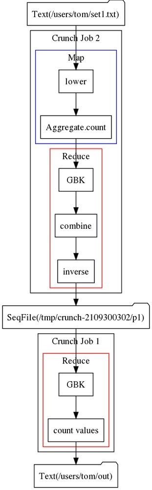
_Figure 18-1. Plan diagram for a Crunch pipeline for calculating a histogram of word counts _After the lowercasing operation, the next transformation in the program is to produce a
PTable of counts of each unique string, using the built-in convenience method count().
This method actually performs three primitive Crunch operations: a parallelDo() named Aggregate.count, a groupByKey() operation labeled GBK in the diagram, and a combineValues() operation labeled combine.
Each GBK operation is realized as a MapReduce shuffle step, with the groupByKey() and combineValues() operations running in the reduce phase. The Aggregate.count parallelDo() operation runs in the map phase, but notice that it is run in the same map as the lower operation: the Crunch planner attempts to minimize the number of MapReduce jobs that it needs to run for a pipeline. In a similar way, the inverse parallelDo() operation is run as a part of the preceding reduce.125]
The last transformation is to take the inverted counts PTable and find the frequency of each count. For example, if the strings that occur three times are apple and orange, then the count of 3 has a frequency of 2. This transformation is another GBK operation, which forces a new MapReduce job (Crunch Job 1), followed by a mapValues() operation that we named count values. The mapValues() operation is simply a parallelDo() operation that can therefore be run in the reduce.
Notice that the map phase for Crunch Job 1 is omitted from the diagram since no primitive Crunch operations are run in it.
Iterative Algorithms
A common use of PObjects is to check for convergence in an iterative algorithm. The classic example of a distributed iterative algorithm is the PageRank algorithm for ranking the relative importance of each of a set of linked pages, such as the World Wide Web.126] The control flow for a Crunch implementation of PageRank looks like this:
PTable
scores = pageRank(scores, 0.5f);
PObject
Without going into detail on the operation of the PageRank algorithm itself, we can understand how the higher-level program execution works in Crunch.
The input is a text file with two URLs per line: a page and an outbound link from that page. For example, the following file encodes the fact that A has links to B and C, and B has
| a link to D: | |
|---|---|
| www.A.com | www.B.com |
| www.A.com | www.C.com |
| www.B.com | www.D.com |
Going back to the code, the first line reads the input and computes an initial PageRankData object for each unique page. PageRankData is a simple Java class with fields for the score, the previous score (this will be used to check for convergence), and a list of outbound links:
public static class PageRankData { public float score; public float lastScore; public List
// … methods elided }
The goal of the algorithm is to compute a score for each page, representing its relative importance. All pages start out equal, so the initial score is set to be 1 for each page, and the previous score is 0. Creating the list of outbound links is achieved using the Crunch operations of grouping the input by the first field (page), then aggregating the values
(outbound links) into a list.127]
The iteration is carried out using a regular Java while loop. The scores are updated in each iteration of the loop by calling the pageRank() method, which encapsulates the PageRank algorithm as a series of Crunch operations. If the delta between the last set of scores and the new set of scores is below a small enough value (0.01), then the scores have converged and the algorithm terminates. The delta is computed by the computeDelta() method, a Crunch aggregation that finds the largest absolute difference in page score for all the pages in the collection.
So when is the pipeline run? The answer is each time pDelta.getValue() is called. The first time through the loop, no PCollections have been materialized yet, so the jobs for readUrls(), pageRank(), and computeDelta() must be run in order to compute delta. On subsequent iterations only the jobs to compute the new scores (pageRank()) and delta (computeDelta()) need be run.
NOTE
For this pipeline, Crunch’s planner does a better job of optimizing the execution plan if scores.materialize().iterator() is called immediately after the pageRank() call. This ensures that the scores table is explicitly materialized, so it is available for the next execution plan in the next iteration of the loop. Without the call to materialize(), the program still produces the same result, but it’s less efficient: the planner may choose to materialize different intermediate results, and so for the next iteration of the loop some of the computation must be reexecuted to get the scores to pass to the pageRank() call.
Checkpointing a Pipeline
In the previous section, we saw that Crunch will reuse any PCollections that were materialized in any previous runs of the same pipeline. However, if you create a new pipeline instance, then it will not automatically share any materialized PCollections from other pipelines, even if the input source is the same. This can make developing a pipeline rather time consuming, since even a small change to a computation toward the end of the pipeline means Crunch will run the new pipeline from the beginning.
The solution is to checkpoint a PCollection to persistent storage (typically HDFS) so that Crunch can start from the checkpoint in the new pipeline.
Consider the Crunch program for calculating a histogram of word counts for text files back in Example 18-3. We saw that the Crunch planner translates this pipeline into two
MapReduce jobs. If the program is run for a second time, then Crunch will run the two MapReduce jobs again and overwrite the original output, since WriteMode is set to OVERWRITE.
If instead we checkpointed inverseCounts, a subsequent run would only launch one MapReduce job (the one for computing hist, since it is entirely derived from inverseCounts). Checkpointing is simply a matter of writing a PCollection to a target
with the WriteMode set to CHECKPOINT:
PCollection
PTable
PTable
new InversePairFn
Target.WriteMode.CHECKPOINT); PTable
.groupByKey()
.mapValues(new CountValuesFn
Crunch compares the timestamps of the input files with those of the checkpoint files; if any inputs have later timestamps than the checkpoints, then it will recompute the dependent checkpoints automatically, so there is no risk of using out-of-date data in the pipeline.
Since they are persistent between pipeline runs, checkpoints are not cleaned up by Crunch, so you will need to delete them once you are happy that the code is producing the expected results.
Crunch Libraries
Crunch comes with a powerful set of library functions in the org.apache.crunch.lib package — they are summarized in Table 18-1.
Table 18-1. Crunch libraries
| Class | Method name(s) | Description |
|---|---|---|
| Aggregate | length() | Returns the number of elements in a PCollection wrapped in a PObject. |
| min() | Returns the smallest value element in a PCollection wrapped in a PObject. | |
| max() | Returns the largest value element in a PCollection wrapped in a PObject. | |
| count() | Returns a table of the unique elements of the input PCollection mapped to their counts. | |
| top() | Returns a table of the top or bottom N key-value pairs in a PTable, ordered by value. | |
| collectValues() | Groups the values for each unique key in a table into a Java Collection, returning a PTable |
|
| Cartesian | cross() | Calculates the cross product of two PCollections or PTables. |
| Channels | split() | Splits a collection of pairs (PCollection |
| Cogroup | cogroup() | Groups the elements in two or more PTables by key. |
| Distinct | distinct() | Creates a new PCollection or PTable with duplicate elements removed. |
Join join() Performs an inner join on two PTables by key. There are also methods for
left, right, and full joins.
| Mapred | map() | Runs a mapper (old API) on a PTable |
|---|---|---|
| reduce() | Runs a reducer (old API) on a PGroupedTable |
|
| Mapreduce | map(), reduce() | Like Mapred, but for the new MapReduce API. |
PTables asPTable() Converts a PCollection
| keys() | Returns a PTable’s keys as a PCollection. |
|---|---|
| values() | Returns a PTable’s values as a PCollection. |
| mapKeys() | Applies a map function to all the keys in a PTable, leaving the values unchanged. |
mapValues() Applies a map function to all the values in a PTable or PGroupedTable, leaving the keys unchanged.
| Sample | sample() | Creates a sample of a PCollection by choosing each element independently with a specified probability. |
|---|---|---|
| reservoirSample() | Creates a sample of a PCollection of a specified size, where each element is equally likely to be included. | |
| SecondarySort | sortAndApply() | Sorts a PTable |
Set difference() Returns a PCollection that is the set difference of two PCollections.
| intersection() | Returns a PCollection that is the set intersection of two PCollections. |
|---|---|

comm() Returns a PCollection of triples that classifies each element from two
PCollections by whether it is only in the first collection, only in the second collection, or in both collections. (Similar to the Unix comm command.)
| Shard | shard() | Creates a PCollection that contains exactly the same elements as the input PCollection, but is partitioned (sharded) across a specified number of files. |
|---|---|---|
Sort sort() Performs a total sort on a PCollection in the natural order of its elements
in ascending (the default) or descending order. There are also methods to sort PTables by key, and collections of Pairs or tuples by a subset of their columns in a specified order.
One of the most powerful things about Crunch is that if the function you need is not provided, then it is simple to write it yourself, typically in a few lines of Java. For an example of a general-purpose function (for finding the unique values in a PTable), see Example 18-2.
The methods length(), min(), max(), and count() from Aggregate have convenience method equivalents on PCollection. Similarly, top() (as well as the derived method bottom()) and collectValues() from Aggregate, all the methods from PTables, join() from Join, and cogroup() from Cogroup are all duplicated on PTable.
The code in Example 18-4 walks through the behavior of some of the aggregation methods.
Example 18-4. Using the aggregation methods on PCollection and PTable
PCollection
“cherry”, “apple”, “banana”, “banana”);
assertEquals((Long) 4L, a.length().getValue()); assertEquals(“apple”, a.min().getValue()); assertEquals(“cherry”, a.max().getValue());
PTable
PTable
PTable
Further Reading
This chapter has given a short introduction to Crunch. To find out more, consult the Crunch User Guide.
[118] Some operations do not require a PType, since they can infer it from the PCollection they are applied to. For example, filter() returns a PCollection with the same PType as the original.
[119] Despite the name, APPEND does not append to existing output files.
[120] HBaseTarget does not check for existing outputs, so it behaves as if APPEND mode is used.
[121] See the documentation.
[122] This is an example of where a pipeline gets executed without an explicit call to run() or done(), but it is still good practice to call done() when the pipeline is finished with so that intermediate files are disposed of.
[123] There is also an asMap() method on PTable
[124] You can increment your own custom counters from Crunch using DoFn’s increment() method.
[125] This optimization is called parallelDo fusion; it explained in more detail in the FlumeJava paper referenced at the beginning of the chapter, along with some of the other optimizations used by Crunch. Note that parallelDo fusion is what allows you to decompose pipeline operations into small, logically separate functions without any loss of efficiency, since Crunch fuses them into as few MapReduce stages as possible.
[126] For details, see Wikipedia.
[127] You can find the full source code in the Crunch integration tests in a class called PageRankIT.
Chapter 19. Spark
Apache Spark is a cluster computing framework for large-scale data processing. Unlike most of the other processing frameworks discussed in this book, Spark does not use MapReduce as an execution engine; instead, it uses its own distributed runtime for executing work on a cluster. However, Spark has many parallels with MapReduce, in terms of both API and runtime, as we will see in this chapter. Spark is closely integrated with Hadoop: it can run on YARN and works with Hadoop file formats and storage backends like HDFS.
Spark is best known for its ability to keep large working datasets in memory between jobs. This capability allows Spark to outperform the equivalent MapReduce workflow (by an order of magnitude or more in some cases128]), where datasets are always loaded from disk. Two styles of application that benefit greatly from Spark’s processing model are iterative algorithms (where a function is applied to a dataset repeatedly until an exit condition is met) and interactive analysis (where a user issues a series of ad hoc exploratory queries on a dataset).
Even if you don’t need in-memory caching, Spark is very attractive for a couple of other reasons: its DAG engine and its user experience. Unlike MapReduce, Spark’s DAG engine can process arbitrary pipelines of operators and translate them into a single job for the user.
Spark’s user experience is also second to none, with a rich set of APIs for performing many common data processing tasks, such as joins. At the time of writing, Spark provides APIs in three languages: Scala, Java, and Python. We’ll use the Scala API for most of the examples in this chapter, but they should be easy to translate to the other languages. Spark also comes with a REPL (read — eval — print loop) for both Scala and Python, which makes it quick and easy to explore datasets.
Spark is proving to be a good platform on which to build analytics tools, too, and to this end the Apache Spark project includes modules for machine learning (MLlib), graph processing (GraphX), stream processing (Spark Streaming), and SQL (Spark SQL). These modules are not covered in this chapter; the interested reader should refer to the Apache Spark website.
Installing Spark
Download a stable release of the Spark binary distribution from the downloads page (choose the one that matches the Hadoop distribution you are using), and unpack the tarball in a suitable location:
% tar xzf spark-x.y.z-bin-distro.tgz
It’s convenient to put the Spark binaries on your path as follows:
% export SPARKHOME=~/sw/spark-_x.y.z-bin-distro
% export PATH=$PATH:$SPARK_HOME/bin
We’re now ready to run an example in Spark.
An Example
To introduce Spark, let’s run an interactive session using spark-shell, which is a Scala REPL with a few Spark additions. Start up the shell with the following:
% spark-shell
Spark context available as sc.
scala>
From the console output, we can see that the shell has created a Scala variable, sc, to store the SparkContext instance. This is our entry point to Spark, and allows us to load a text file as follows:
scala> val lines = sc.textFile(“input/ncdc/micro-tab/sample.txt”) lines: org.apache.spark.rdd.RDD[String] = MappedRDD[1] at textFile at
The lines variable is a reference to a Resilient Distributed Dataset, abbreviated to RDD, which is the central abstraction in Spark: a read-only collection of objects that is partitioned across multiple machines in a cluster. In a typical Spark program, one or more RDDs are loaded as input and through a series of transformations are turned into a set of target RDDs, which have an action performed on them (such as computing a result or writing them to persistent storage). The term “resilient” in “Resilient Distributed Dataset” refers to the fact that Spark can automatically reconstruct a lost partition by recomputing it from the RDDs that it was computed from.
the lines into fields:
scala> val records = lines.map(_.split(“\t”)) records: org.apache.spark.rdd.RDD[Array[String]] = MappedRDD[2] at map at
This uses the map() method on RDD to apply a function to every element in the RDD. In this case, we split each line (a String) into a Scala Array of Strings.
Next, we apply a filter to remove any bad records:
scala> val filtered = records.filter(rec => (rec(1) != “9999”
&& rec(2).matches(“[01459]”))) filtered: org.apache.spark.rdd.RDD[Array[String]] = FilteredRDD[3] at filter at
The filter() method on RDD takes a predicate, a function that returns a Boolean. This one tests for records that don’t have a missing temperature (indicated by 9999) or a bad quality reading.
To find the maximum temperatures for each year, we need to perform a grouping operation on the year field so we can process all the temperature values for each year.
Spark provides a reduceByKey() method to do this, but it needs an RDD of key-value pairs, represented by a Scala Tuple2. So, first we need to transform our RDD into the correct form using another map:
scala> val tuples = filtered.map(rec => (rec(0).toInt, rec(1).toInt)) tuples: org.apache.spark.rdd.RDD[(Int, Int)] = MappedRDD[4] at map at
Then we can perform the aggregation. The reduceByKey() method’s argument is a function that takes a pair of values and combines them into a single value; in this case, we use Java’s Math.max function:
scala> val maxTemps = tuples.reduceByKey((a, b) => Math.max(a, b)) maxTemps: org.apache.spark.rdd.RDD[(Int, Int)] = MapPartitionsRDD[7] at reduceByKey at
We can display the contents of maxTemps by invoking the foreach() method and passing println() to print each element to the console:
scala> maxTemps.foreach(println(_))
(1950,22)
(1949,111)
The foreach() method is the same as the equivalent on standard Scala collections, like List, and applies a function (that has some side effect) to each element in the RDD. It is this operation that causes Spark to run a job to compute the values in the RDD, so they can be run through the println() method.
Alternatively, we can save the RDD to the filesystem with: scala> maxTemps.saveAsTextFile(“output”)
which creates a directory called output containing the partition files:
% cat output/part-*
(1950,22)
(1949,111)
The saveAsTextFile() method also triggers a Spark job. The main difference is that no value is returned, and instead the RDD is computed and its partitions are written to files in the output directory.
Spark Applications, Jobs, Stages, and Tasks
As we’ve seen in the example, like MapReduce, Spark has the concept of a job. A Spark job is more general than a MapReduce job, though, since it is made up of an arbitrary directed acyclic graph (DAG) of stages, each of which is roughly equivalent to a map or reduce phase in MapReduce.
Stages are split into tasks by the Spark runtime and are run in parallel on partitions of an RDD spread across the cluster — just like tasks in MapReduce.
A job always runs in the context of an application (represented by a SparkContext instance) that serves to group RDDs and shared variables. An application can run more than one job, in series or in parallel, and provides the mechanism for a job to access an RDD that was cached by a previous job in the same application. (We will see how to cache RDDs in Persistence.) An interactive Spark session, such as a spark-shell session, is just an instance of an application.
A Scala Standalone Application
After working with the Spark shell to refine a program, you may want to package it into a
self-contained application that can be run more than once. The Scala program in Example 19-1 shows how to do this.
Example 19-1. Scala application to find the maximum temperature, using Spark
import org.apache.spark.SparkContext._ import org.apache.spark.{SparkConf, SparkContext}
object MaxTemperature { def main(args: Array[String]) { val conf = new SparkConf().setAppName(“Max Temperature”) val sc = new SparkContext(conf)
sc.textFile(args(0))
.map(_.split(“\t”))
.filter(rec => (rec(1) != “9999” && rec(2).matches(“[01459]”)))
.map(rec => (rec(0).toInt, rec(1).toInt)) .reduceByKey((a, b) => Math.max(a, b))
.saveAsTextFile(args(1))
} }
When running a standalone program, we need to create the SparkContext since there is no shell to provide it. We create a new instance with a SparkConf, which allows us to pass various Spark properties to the application; here we just set the application name.
There are a couple of other minor changes. The first is that we’ve used the command-line arguments to specify the input and output paths. We’ve also used method chaining to avoid having to create intermediate variables for each RDD. This makes the program more compact, and we can still view the type information for each transformation in the Scala IDE if needed.
NOTE
Not all the transformations that Spark defines are available on the RDD class itself. In this case, reducebyKey() (which acts only on RDDs of key-value pairs) is actually defined in the PairRDDFunctions class, but we can get Scala to implicitly convert RDD[(Int, Int)] to PairRDDFunctions with the following import: import org.apache.spark.SparkContext._
This imports various implicit conversion functions used in Spark, so it is worth including in programs as a matter of course.
This time we use spark-submit to run the program, passing as arguments the application JAR containing the compiled Scala program, followed by our program’s command-line arguments (the input and output paths):
% spark-submit —class MaxTemperature —master local \ spark-examples.jar input/ncdc/micro-tab/sample.txt output % cat output/part-*
(1950,22)
(1949,111)
We also specified two options: —class to tell Spark the name of the application class, and
—master to specify where the job should run. The value local tells Spark to run everything in a single JVM on the local machine. We’ll learn about the options for running on a cluster in Executors and Cluster Managers. Next, let’s see how to use other languages with Spark, starting with Java.
A Java Example
Spark is implemented in Scala, which as a JVM-based language has excellent integration with Java. It is straightforward — albeit verbose — to express the same example in Java (see Example 19-2).129]
Example 19-2. Java application to find the maximum temperature, using Spark
public class MaxTemperatureSpark {
public static void main(String[] args) throws Exception { if (args.length != 2) {
System.err.println(“Usage: MaxTemperatureSpark
Example 19-3. Python application to find the maximum temperature, using PySpark
from pyspark import SparkContext import re, sys
sc = SparkContext(“local”, “Max Temperature”) sc.textFile(sys.argv[1]) \
.map(lambda s: s.split(“\t“)) \
.filter(lambda rec: (rec[1] != “9999” and re.match(“[01459]”, rec[2]))) \
.map(lambda rec: (int(rec[0]), int(rec[1]))) \
.reduceByKey(max) \
.saveAsTextFile(sys.argv[2])
Notice that for the reduceByKey() transformation we can use Python’s built-in max function.
The important thing to note is that this program is written in regular CPython. Spark will fork Python subprocesses to run the user’s Python code (both in the launcher program and on executors that run user tasks in the cluster), and uses a socket to connect the two processes so the parent can pass RDD partition data to be processed by the Python code.
To run, we specify the Python file rather than the application JAR:
% spark-submit —master local \
ch19-spark/src/main/python/MaxTemperature.py \ input/ncdc/micro-tab/sample.txt output
Spark can also be run with Python in interactive mode using the pyspark command.
Resilient Distributed Datasets
RDDs are at the heart of every Spark program, so in this section we look at how to work with them in more detail.
Creation
There are three ways of creating RDDs: from an in-memory collection of objects (known as parallelizing a collection), using a dataset from external storage (such as HDFS), or transforming an existing RDD. The first way is useful for doing CPU-intensive computations on small amounts of input data in parallel. For example, the following runs separate computations on the numbers from 1 to 10:130]
val params = sc.parallelize(1 to 10) val result = params.map(performExpensiveComputation)
The performExpensiveComputation function is run on input values in parallel. The level of parallelism is determined from the spark.default.parallelism property, which has a default value that depends on where the Spark job is running. When running locally it is the number of cores on the machine, while for a cluster it is the total number of cores on all executor nodes in the cluster.
You can also override the level of parallelism for a particular computation by passing it as the second argument to parallelize(): sc.parallelize(1 to 10, 10)
The second way to create an RDD is by creating a reference to an external dataset. We have already seen how to create an RDD of String objects for a text file: val text: RDD[String] = sc.textFile(inputPath)
The path may be any Hadoop filesystem path, such as a file on the local filesystem or on
HDFS. Internally, Spark uses TextInputFormat from the old MapReduce API to read the file (see TextInputFormat). This means that the file-splitting behavior is the same as in Hadoop itself, so in the case of HDFS there is one Spark partition per HDFS block. The default can be changed by passing a second argument to request a particular number of splits: sc.textFile(inputPath, 10)
Another variant permits text files to be processed as whole files (similar to Processing a whole file as a record) by returning an RDD of string pairs, where the first string is the file path and the second is the file contents. Since each file is loaded into memory, this is only suitable for small files: val files: RDD[(String, String)] = sc.wholeTextFiles(inputPath)
Spark can work with other file formats besides text. For example, sequence files can be read with: sc.sequenceFileIntWritable, Text
Notice how the sequence file’s key and value Writable types have been specified. For common Writable types, Spark can map them to the Java equivalents, so we could use the equivalent form:
sc.sequenceFileInt, String
There are two methods for creating RDDs from an arbitrary Hadoop InputFormat:
hadoopFile() for file-based formats that expect a path, and hadoopRDD() for those that don’t, such as HBase’s TableInputFormat. These methods are for the old MapReduce API; for the new one, use newAPIHadoopFile() and newAPIHadoopRDD(). Here is an example of reading an Avro datafile using the Specific API with a WeatherRecord class:
val job = new Job()
AvroJob.setInputKeySchema(job, WeatherRecord.getClassSchema) val data = sc.newAPIHadoopFile(inputPath, classOf[AvroKeyInputFormat[WeatherRecord]], classOf[AvroKey[WeatherRecord]], classOf[NullWritable], job.getConfiguration)
In addition to the path, the newAPIHadoopFile() method expects the InputFormat type, the key type, and the value type, plus the Hadoop configuration. The configuration carries the Avro schema, which we set in the second line using the AvroJob helper class.
The third way of creating an RDD is by transforming an existing RDD. We look at transformations next.
Transformations and Actions
Spark provides two categories of operations on RDDs: transformations and actions. A transformation generates a new RDD from an existing one, while an action triggers a computation on an RDD and does something with the results — either returning them to the user, or saving them to external storage.
Actions have an immediate effect, but transformations do not — they are lazy, in the sense that they don’t perform any work until an action is performed on the transformed RDD. For example, the following lowercases lines in a text file:
val text = sc.textFile(inputPath)
val lower: RDD[String] = text.map(_.toLowerCase()) lower.foreach(println(_))
The map() method is a transformation, which Spark represents internally as a function
(toLowerCase()) to be called at some later time on each element in the input RDD (text). The function is not actually called until the foreach() method (which is an action) is invoked and Spark runs a job to read the input file and call toLowerCase() on each line in it, before writing the result to the console.
One way of telling if an operation is a transformation or an action is by looking at its return type: if the return type is RDD, then it’s a transformation; otherwise, it’s an action. It’s useful to know this when looking at the documentation for RDD (in the
org.apache.spark.rdd package), where most of the operations that can be performed on RDDs can be found. More operations can be found in PairRDDFunctions, which contains transformations and actions for working with RDDs of key-value pairs.
Spark’s library contains a rich set of operators, including transformations for mapping, grouping, aggregating, repartitioning, sampling, and joining RDDs, and for treating RDDs as sets. There are also actions for materializing RDDs as collections, computing statistics on RDDs, sampling a fixed number of elements from an RDD, and saving RDDs to external storage. For details, consult the class documentation.
MAPREDUCE IN SPARK
Despite the suggestive naming, Spark’s map() and reduce() operations do not directly correspond to the functions of the same name in Hadoop MapReduce. The general form of map and reduce in Hadoop MapReduce is (from Chapter 8):
map: (K1, V1) → list(K2, V2) reduce: (K2, list(V2)) → list(K3, V3)
Notice that both functions can return multiple output pairs, indicated by the list notation. This is implemented by the flatMap() operation in Spark (and Scala in general), which is like map(), but removes a layer of nesting:
scala> val l = List(1, 2, 3) l: List[Int] = List(1, 2, 3)
scala> l.map(a => List(a))
res0: List[List[Int]] = List(List(1), List(2), List(3))
scala> l.flatMap(a => List(a)) res1: List[Int] = List(1, 2, 3)
One naive way to try to emulate Hadoop MapReduce in Spark is with two flatMap() operations, separated by a groupByKey() and a sortByKey() to perform a MapReduce shuffle and sort:
val input: RDD[(K1, V1)] = …
val mapOutput: RDD[(K2, V2)] = input.flatMap(mapFn) val shuffled: RDD[(K2, Iterable[V2])] = mapOutput.groupByKey().sortByKey() val output: RDD[(K3, V3)] = shuffled.flatMap(reduceFn)
Here the key type K2 needs to inherit from Scala’s Ordering type to satisfy sortByKey().
This example may be useful as a way to help understand the relationship between MapReduce and Spark, but it should not be applied blindly. For one thing, the semantics are slightly different from Hadoop’s MapReduce, since sortByKey() performs a total sort. This issue can be avoided by using repartitionAndSortWithinPartitions() to perform a partial sort. However, even this isn’t as efficient, since Spark uses two shuffles (one for the groupByKey() and one for the sort).
Rather than trying to reproduce MapReduce, it is better to use only the operations that you actually need. For example, if you don’t need keys to be sorted, you can omit the sortByKey() call (something that is not possible in regular Hadoop MapReduce).
Similarly, groupByKey() is too general in most cases. Usually you only need the shuffle to aggregate values, so you should use reduceByKey(), foldByKey(), or aggregateByKey() (covered in the next section), which are more efficient than groupByKey() since they can also run as combiners in the map task. Finally, flatMap() may not always be needed either, with map() being preferred if there is always one return value, and filter() if there is zero or one.
Aggregation transformations
The three main transformations for aggregating RDDs of pairs by their keys are reduceByKey(), foldByKey(), and aggregateByKey(). They work in slightly different ways, but they all aggregate the values for a given key to produce a single value for each key. (The equivalent actions are reduce(), fold(), and aggregate(), which operate in an analogous way, resulting in a single value for the whole RDD.)
The simplest is reduceByKey(), which repeatedly applies a binary function to values in pairs until a single value is produced. For example:
val pairs: RDD[(String, Int)] = sc.parallelize(Array((“a”, 3), (“a”, 1), (“b”, 7), (“a”, 5))) val sums: RDD[(String, Int)] = pairs.reduceByKey(_+_) assert(sums.collect().toSet === Set((“a”, 9), (“b”, 7)))
The values for key a are aggregated using the addition function (+) as (3 + 1) + 5 = 9, while there is only one value for key b, so no aggregation is needed. Since in general the operations are distributed and performed in different tasks for different partitions of the RDD, the function should be commutative and associative. In other words, the order and grouping of the operations should not matter; in this case, the aggregation could be 5 + (3 + 1), or 3 + (1 + 5), which both return the same result.
Here’s how we would perform the same operation using foldByKey():
val sums: RDD[(String, Int)] = pairs.foldByKey(0)(_+_) assert(sums.collect().toSet === Set((“a”, 9), (“b”, 7)))
Notice that this time we had to supply a zero value, which is just 0 when adding integers, but would be something different for other types and operations. This time, values for a are aggregated as ((0 + 3) + 1) + 5) = 9 (or possibly some other order, although adding to 0 is always the first operation). For b it is 0 + 7 = 7.
Using foldByKey() is no more or less powerful than using reduceByKey(). In particular, neither can change the type of the value that is the result of the aggregation. For that we need aggregateByKey(). For example, we can aggregate the integer values into a set:
val sets: RDD[(String, HashSet[Int])] = pairs.aggregateByKey(new HashSet[Int])(_+=_, _++=_) assert(sets.collect().toSet === Set((“a”, Set(1, 3, 5)), (“b”, Set(7))))
For set addition, the zero value is the empty set, so we create a new mutable set with new
HashSet[Int]. We have to supply two functions to aggregateByKey(). The first controls how an Int is combined with a HashSet[Int], and in this case we use the addition and assignment function += to add the integer to the set (+ would return a new set and leave the first set unchanged).
The second function controls how two HashSet[Int] values are combined (this happens after the combiner runs in the map task, while the two partitions are being aggregated in the reduce task), and here we use ++= to add all the elements of the second set to the first.
For key a, the sequence of operations might be:
((∅ + 3) + 1) + 5) = (1, 3, 5) _or:
(∅ + 3) + 1) ++ (∅ + 5) = (1, 3) ++ (5) = (1, 3, 5) _if Spark uses a combiner.
A transformed RDD can be persisted in memory so that subsequent operations on it are more efficient. We look at that next.
Persistence
Going back to the introductory example in An Example, we can cache the intermediate dataset of year-temperature pairs in memory with the following:
scala> tuples.cache() res1: tuples.type = MappedRDD[4] at map at
Calling cache() does not cache the RDD in memory straightaway. Instead, it marks the RDD with a flag indicating it should be cached when the Spark job is run. So let’s first force a job run:
scala> tuples.reduceByKey((a, b) => Math.max(a, b)).foreach(println(_))
INFO BlockManagerInfo: Added rdd4_0 in memory on 192.168.1.90:64640 INFO BlockManagerInfo: Added rdd_4_1 in memory on 192.168.1.90:64640
(1950,22)
(1949,111)
The log lines for BlockManagerInfo show that the RDD’s partitions have been kept in memory as a part of the job run. The log shows that the RDD’s number is 4 (this was shown in the console after calling the cache() method), and it has two partitions labeled 0 and 1. If we run another job on the cached dataset, we’ll see that the RDD is loaded from memory. This time we’ll compute minimum temperatures:
scala> **tuples.reduceByKey((a, b) => Math.min(a, b)).foreach(println())
INFO BlockManager: Found block rdd_4_0 locally
INFO BlockManager: Found block rdd_4_1 locally
(1949,78)
(1950,-11)
This is a simple example on a tiny dataset, but for larger jobs the time savings can be impressive. Compare this to MapReduce, where to perform another calculation the input dataset has to be loaded from disk again. Even if an intermediate dataset can be used as input (such as a cleaned-up dataset with invalid rows and unnecessary fields removed), there is no getting away from the fact that it must be loaded from disk, which is slow. Spark will cache datasets in a cross-cluster in-memory cache, which means that any computation performed on those datasets will be very fast.
This turns out to be tremendously useful for interactive exploration of data. It’s also a natural fit for certain styles of algorithm, such as iterative algorithms where a result computed in one iteration can be cached in memory and used as input for the next iteration. These algorithms can be expressed in MapReduce, but each iteration runs as a single MapReduce job, so the result from each iteration must be written to disk and then read back in the next iteration.
NOTE*
Cached RDDs can be retrieved only by jobs in the same application. To share datasets between applications, they must be written to external storage using one of the saveAs() methods (saveAsTextFile(), saveAsHadoopFile(), etc.) in the first application, then loaded using the corresponding method in SparkContext (textFile(), hadoopFile(), etc.) in the second application. Likewise, when the application terminates, all its cached RDDs are destroyed and cannot be accessed again unless they have been explicitly saved.
Persistence levels
Calling cache() will persist each partition of the RDD in the executor’s memory. If an executor does not have enough memory to store the RDD partition, the computation will not fail, but instead the partition will be recomputed as needed. For complex programs with lots of transformations, this may be expensive, so Spark offers different types of persistence behavior that may be selected by calling persist() with an argument to specify the StorageLevel.
By default, the level is MEMORY_ONLY, which uses the regular in-memory representation of objects. A more compact representation can be used by serializing the elements in a partition as a byte array. This level is MEMORY_ONLY_SER; it incurs CPU overhead compared to MEMORY_ONLY, but is worth it if the resulting serialized RDD partition fits in memory when the regular in-memory representation doesn’t. MEMORY_ONLY_SER also reduces garbage collection pressure, since each RDD is stored as one byte array rather than lots of objects.
NOTE
You can see if an RDD partition doesn’t fit in memory by inspecting the driver logfile for messages from the
BlockManager. Also, every driver’s SparkContext runs an HTTP server (on port 4040) that provides useful information about its environment and the jobs it is running, including information about cached RDD partitions.
By default, regular Java serialization is used to serialize RDD partitions, but Kryo serialization (covered in the next section) is normally a better choice, both in terms of size and speed. Further space savings can be achieved (again at the expense of CPU) by compressing the serialized partitions by setting the spark.rdd.compress property to true, and optionally setting spark.io.compression.codec.
If recomputing a dataset is expensive, then either MEMORY_AND_DISK (spill to disk if the dataset doesn’t fit in memory) or MEMORY_AND_DISK_SER (spill to disk if the serialized dataset doesn’t fit in memory) is appropriate.
There are also some more advanced and experimental persistence levels for replicating partitions on more than one node in the cluster, or using off-heap memory — see the Spark documentation for details.
Serialization
There are two aspects of serialization to consider in Spark: serialization of data and serialization of functions (or closures).
Data
Let’s look at data serialization first. By default, Spark will use Java serialization to send data over the network from one executor to another, or when caching (persisting) data in serialized form as described in Persistence levels. Java serialization is well understood by programmers (you make sure the class you are using implements java.io.Serializable or java.io.Externalizable), but it is not particularly efficient from a performance or size perspective.
A better choice for most Spark programs is Kryo serialization. Kryo is a more efficient general-purpose serialization library for Java. In order to use Kryo serialization, set the spark.serializer as follows on the SparkConf in your driver program: conf.set(“spark.serializer”, “org.apache.spark.serializer.KryoSerializer”) Kryo does not require that a class implement a particular interface (like java.io.Serializable) to be serialized, so plain old Java objects can be used in RDDs without any further work beyond enabling Kryo serialization. Having said that, it is much more efficient to register classes with Kryo before using them. This is because Kryo writes a reference to the class of the object being serialized (one reference is written for every object written), which is just an integer identifier if the class has been registered but is the full classname otherwise. This guidance only applies to your own classes; Spark registers Scala classes and many other framework classes (like Avro Generic or Thrift classes) on your behalf.
Registering classes with Kryo is straightforward. Create a subclass of KryoRegistrator, and override the registerClasses() method:
class CustomKryoRegistrator extends KryoRegistrator { override def registerClasses(kryo: Kryo) { kryo.register(classOf[WeatherRecord])
} }
Finally, in your driver program, set the spark.kryo.registrator property to the fully qualified classname of your KryoRegistrator implementation: conf.set(“spark.kryo.registrator”, “CustomKryoRegistrator”)
Functions
Generally, serialization of functions will “just work”: in Scala, functions are serializable using the standard Java serialization mechanism, which is what Spark uses to send functions to remote executor nodes. Spark will serialize functions even when running in local mode, so if you inadvertently introduce a function that is not serializable (such as one converted from a method on a nonserializable class), you will catch it early on in the development process.
Shared Variables
Spark programs often need to access data that is not part of an RDD. For example, this program uses a lookup table in a map() operation:
val lookup = Map(1 -> “a”, 2 -> “e”, 3 -> “i”, 4 -> “o”, 5 -> “u”) val result = sc.parallelize(Array(2, 1, 3)).map(lookup(_)) assert(result.collect().toSet === Set(“a”, “e”, “i”))
While it works correctly (the variable lookup is serialized as a part of the closure passed to map()), there is a more efficient way to achieve the same thing using broadcast variables.
Broadcast Variables
A broadcast variable is serialized and sent to each executor, where it is cached so that later tasks can access it if needed. This is unlike a regular variable that is serialized as part of the closure, which is transmitted over the network once per task. Broadcast variables play a similar role to the distributed cache in MapReduce (see Distributed Cache), although the implementation in Spark stores the data in memory, only spilling to disk when memory is exhausted.
A broadcast variable is created by passing the variable to be broadcast to the broadcast() method on SparkContext. It returns a Broadcast[T] wrapper around the variable of type T:
val lookup: Broadcast[Map[Int, String]] =
sc.broadcast(Map(1 -> “a”, 2 -> “e”, 3 -> “i”, 4 -> “o”, 5 -> “u”)) **val result = sc.parallelize(Array(2, 1, 3)).map(lookup.value(_)) assert(result.collect().toSet === Set**(“a”, “e”, “i”))
Notice that the variable is accessed in the RDD map() operation by calling value on the broadcast variable.
As the name suggests, broadcast variables are sent one way, from driver to task — there is no way to update a broadcast variable and have the update propagate back to the driver. For that, we need an accumulator.
Accumulators
An accumulator is a shared variable that tasks can only add to, like counters in
MapReduce (see Counters). After a job has completed, the accumulator’s final value can be retrieved from the driver program. Here is an example that counts the number of elements in an RDD of integers using an accumulator, while at the same time summing the values in the RDD using a reduce() action:
val count: Accumulator[Int] = sc.accumulator(0) val result = sc.parallelize(Array(1, 2, 3))
.map(i => { count += 1; i }) .reduce((x, y) => x + y) assert(count.value === 3) assert(result === 6)
An accumulator variable, count, is created in the first line using the accumulator() method on SparkContext. The map() operation is an identity function with a side effect that increments count. When the result of the Spark job has been computed, the value of the accumulator is accessed by calling value on it.
In this example, we used an Int for the accumulator, but any numeric value type can be used. Spark also provides a way to use accumulators whose result type is different to the type being added (see the accumulable() method on SparkContext), and a way to accumulate values in mutable collections (via accumulableCollection()).
Anatomy of a Spark Job Run
Let’s walk through what happens when we run a Spark job. At the highest level, there are two independent entities: the driver, which hosts the application (SparkContext) and schedules tasks for a job; and the executors, which are exclusive to the application, run for the duration of the application, and execute the application’s tasks. Usually the driver runs as a client that is not managed by the cluster manager and the executors run on machines in the cluster, but this isn’t always the case (as we’ll see in Executors and Cluster Managers). For the remainder of this section, we assume that the application’s executors are already running.
Job Submission
Figure 19-1 illustrates how Spark runs a job. A Spark job is submitted automatically when an action (such as count()) is performed on an RDD. Internally, this causes runJob() to be called on the SparkContext (step 1 in Figure 19-1), which passes the call on to the scheduler that runs as a part of the driver (step 2). The scheduler is made up of two parts: a DAG scheduler that breaks down the job into a DAG of stages, and a task scheduler that is responsible for submitting the tasks from each stage to the cluster.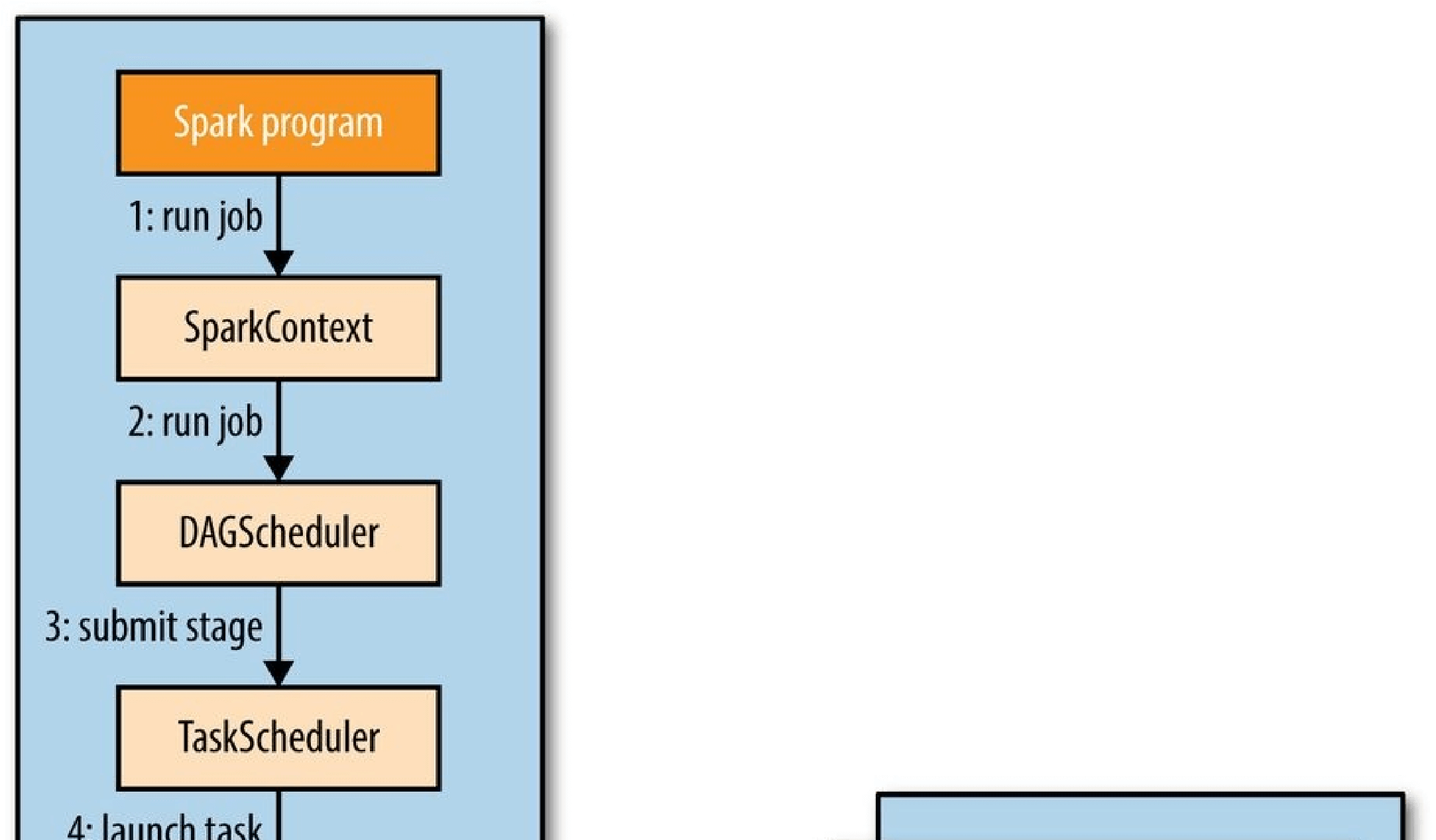
Figure 19-1. How Spark runs a job
Next, let’s take a look at how the DAG scheduler constructs a DAG.
DAG Construction
To understand how a job is broken up into stages, we need to look at the type of tasks that can run in a stage. There are two types: shuffle map tasks and result tasks. The name of the task type indicates what Spark does with the task’s output:
Shuffle map tasks
As the name suggests, shuffle map tasks are like the map-side part of the shuffle in MapReduce. Each shuffle map task runs a computation on one RDD partition and, based on a partitioning function, writes its output to a new set of partitions, which are then fetched in a later stage (which could be composed of either shuffle map tasks or result tasks). Shuffle map tasks run in all stages except the final stage.
Result tasks
Result tasks run in the final stage that returns the result to the user’s program (such as the result of a count()). Each result task runs a computation on its RDD partition, then sends the result back to the driver, and the driver assembles the results from each partition into a final result (which may be Unit, in the case of actions like saveAsTextFile()).
The simplest Spark job is one that does not need a shuffle and therefore has just a single stage composed of result tasks. This is like a map-only job in MapReduce.
More complex jobs involve grouping operations and require one or more shuffle stages. For example, consider the following job for calculating a histogram of word counts for text files stored in inputPath (one word per line):
val hist: Map[Int, Long] = sc.textFile(inputPath)
.map(word => (word.toLowerCase(), 1))
.reduceByKey((a, b) => a + b)
.map(_.swap)
.countByKey()
The first two transformations, map() and reduceByKey(), perform a word count. The third transformation is a map() that swaps the key and value in each pair, to give (count, word) pairs, and the final operation is the countByKey() action, which returns the number of words with each count (i.e., a frequency distribution of word counts).
Spark’s DAG scheduler turns this job into two stages since the reduceByKey() operation forces a shuffle stage.131] The resulting DAG is illustrated in Figure 19-2.
The RDDs within each stage are also, in general, arranged in a DAG. The diagram shows the type of the RDD and the operation that created it. RDD[String] was created by textFile(), for instance. To simplify the diagram, some intermediate RDDs generated internally by Spark have been omitted. For example, the RDD returned by textFile() is actually a MappedRDD[String] whose parent is a HadoopRDD[LongWritable, Text].
Notice that the reduceByKey() transformation spans two stages; this is because it is implemented using a shuffle, and the reduce function runs as a combiner on the map side (stage 1) and as a reducer on the reduce side (stage 2) — just like in MapReduce. Also like MapReduce, Spark’s shuffle implementation writes its output to partitioned files on local disk (even for in-memory RDDs), and the files are fetched by the RDD in the next stage.
[132]
Figure 19-2. The stages and RDDs in a Spark job for calculating a histogram of word counts
If an RDD has been persisted from a previous job in the same application (SparkContext), then the DAG scheduler will save work and not create stages for recomputing it (or the RDDs it was derived from).
The DAG scheduler is responsible for splitting a stage into tasks for submission to the task scheduler. In this example, in the first stage one shuffle map task is run for each partition of the input file. The level of parallelism for a reduceByKey() operation can be set explicitly by passing it as the second parameter. If not set, it will be determined from the parent RDD, which in this case is the number of partitions in the input data.
Each task is given a placement preference by the DAG scheduler to allow the task scheduler to take advantage of data locality. A task that processes a partition of an input RDD stored on HDFS, for example, will have a placement preference for the datanode hosting the partition’s block (known as node local), while a task that processes a partition of an RDD that is cached in memory will prefer the executor storing the RDD partition (process local).
Going back to Figure 19-1, once the DAG scheduler has constructed the complete DAG of stages, it submits each stage’s set of tasks to the task scheduler (step 3). Child stages are only submitted once their parents have completed successfully.
Task Scheduling
When the task scheduler is sent a set of tasks, it uses its list of executors that are running for the application and constructs a mapping of tasks to executors that takes placement preferences into account. Next, the task scheduler assigns tasks to executors that have free cores (this may not be the complete set if another job in the same application is running), and it continues to assign more tasks as executors finish running tasks, until the task set is complete. Each task is allocated one core by default, although this can be changed by setting spark.task.cpus.
Note that for a given executor the scheduler will first assign process-local tasks, then node-local tasks, then rack-local tasks, before assigning an arbitrary (nonlocal) task, or a speculative task if there are no other candidates.133]
Assigned tasks are launched through a scheduler backend (step 4 in Figure 19-1), which sends a remote launch task message (step 5) to the executor backend to tell the executor to run the task (step 6).
Executors also send status update messages to the driver when a task has finished or if a task fails. In the latter case, the task scheduler will resubmit the task on another executor. It will also launch speculative tasks for tasks that are running slowly, if this is enabled (it is not by default).
Task Execution
An executor runs a task as follows (step 7). First, it makes sure that the JAR and file dependencies for the task are up to date. The executor keeps a local cache of all the dependencies that previous tasks have used, so that it only downloads them when they have changed. Second, it deserializes the task code (which includes the user’s functions) from the serialized bytes that were sent as a part of the launch task message. Third, the task code is executed. Note that tasks are run in the same JVM as the executor, so there is no process overhead for task launch.134]
Tasks can return a result to the driver. The result is serialized and sent to the executor backend, and then back to the driver as a status update message. A shuffle map task returns information that allows the next stage to retrieve the output partitions, while a result task returns the value of the result for the partition it ran on, which the driver assembles into a final result to return to the user’s program.
Executors and Cluster Managers
We have seen how Spark relies on executors to run the tasks that make up a Spark job, but we glossed over how the executors actually get started. Managing the lifecycle of executors is the responsibility of the cluster manager, and Spark provides a variety of cluster managers with different characteristics:
Local
In local mode there is a single executor running in the same JVM as the driver. This mode is useful for testing or running small jobs. The master URL for this mode is local
(use one thread), local[n] (n threads), or local(*) (one thread per core on the machine).
Standalone
The standalone cluster manager is a simple distributed implementation that runs a single Spark master and one or more workers. When a Spark application starts, the master will ask the workers to spawn executor processes on behalf of the application. The master
URL is spark://host:port.
Mesos
Apache Mesos is a general-purpose cluster resource manager that allows fine-grained sharing of resources across different applications according to an organizational policy. By default (fine-grained mode), each Spark task is run as a Mesos task. This uses the cluster resources more efficiently, but at the cost of additional process launch overhead. In coarse-grained mode, executors run their tasks in-process, so the cluster resources are held by the executor processes for the duration of the Spark application. The master URL is mesos://host:port.
YARN
YARN is the resource manager used in Hadoop (see Chapter 4). Each running Spark application corresponds to an instance of a YARN application, and each executor runs in its own YARN container. The master URL is yarn-client or yarn-cluster.
The Mesos and YARN cluster managers are superior to the standalone manager since they take into account the resource needs of other applications running on the cluster (MapReduce jobs, for example) and enforce a scheduling policy across all of them. The standalone cluster manager uses a static allocation of resources from the cluster, and therefore is not able to adapt to the varying needs of other applications over time. Also, YARN is the only cluster manager that is integrated with Hadoop’s Kerberos security mechanisms (see Security).
Spark on YARN
Running Spark on YARN provides the tightest integration with other Hadoop components and is the most convenient way to use Spark when you have an existing Hadoop cluster. Spark offers two deploy modes for running on YARN: YARN client mode, where the driver runs in the client, and YARN cluster mode, where the driver runs on the cluster in the YARN application master.
YARN client mode is required for programs that have any interactive component, such as spark-shell or pyspark. Client mode is also useful when building Spark programs, since any debugging output is immediately visible.
YARN cluster mode, on the other hand, is appropriate for production jobs, since the entire application runs on the cluster, which makes it much easier to retain logfiles (including those from the driver program) for later inspection. YARN will also retry the application if the application master fails (see Application Master Failure).
YARN client mode
In YARN client mode, the interaction with YARN starts when a new SparkContext instance is constructed by the driver program (step 1 in Figure 19-3). The context submits a YARN application to the YARN resource manager (step 2), which starts a YARN container on a node manager in the cluster and runs a Spark ExecutorLauncher application master in it (step 3). The job of the ExecutorLauncher is to start executors in YARN containers, which it does by requesting resources from the resource manager (step
4), then launching ExecutorBackend processes as the containers are allocated to it (step 5).
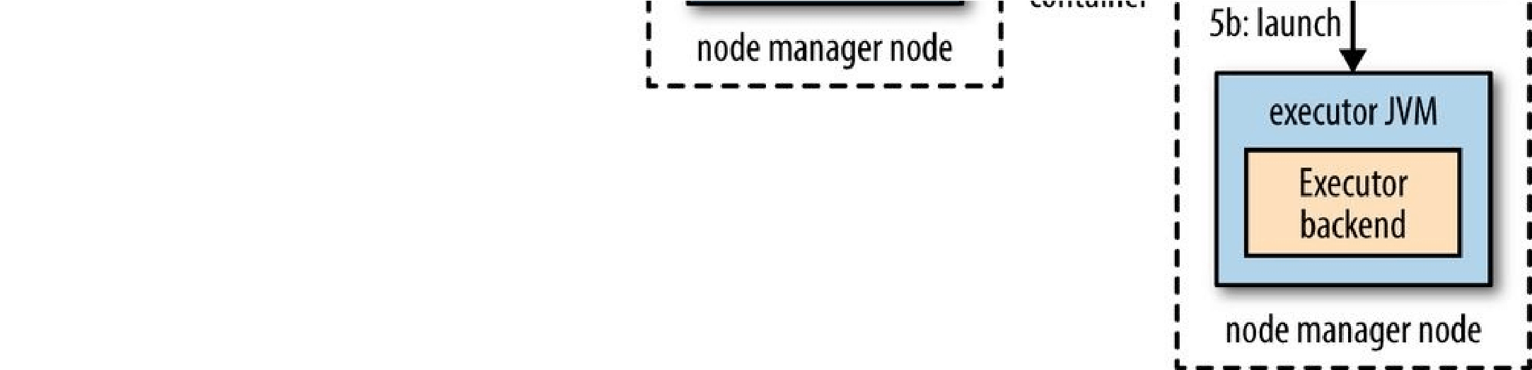
Figure 19-3. How Spark executors are started in YARN client mode
As each executor starts, it connects back to the SparkContext and registers itself. This gives the SparkContext information about the number of executors available for running tasks and their locations, which is used for making task placement decisions (described in Task Scheduling).
The number of executors that are launched is set in spark-shell, spark-submit, or pyspark (if not set, it defaults to two), along with the number of cores that each executor uses (the default is one) and the amount of memory (the default is 1,024 MB). Here’s an example showing how to run spark-shell on YARN with four executors, each using one core and 2 GB of memory:
% spark-shell —master yarn-client \
—num-executors 4 \
—executor-cores 1 \
—executor-memory 2g
The YARN resource manager address is not specified in the master URL (unlike when using the standalone or Mesos cluster managers), but is picked up from Hadoop configuration in the directory specified by the HADOOP_CONF_DIR environment variable.
YARN cluster mode
In YARN cluster mode, the user’s driver program runs in a YARN application master process. The spark-submit command is used with a master URL of yarn-cluster:
% spark-submit —master yarn-cluster…
All other parameters, like —num-executors and the application JAR (or Python file), are the same as for YARN client mode (use spark-submit —help for usage).
The spark-submit client will launch the YARN application (step 1 in Figure 19-4), but it doesn’t run any user code. The rest of the process is the same as client mode, except the application master starts the driver program (step 3b) before allocating resources for executors (step 4).
Figure 19-4. How Spark executors are started in YARN cluster mode
In both YARN modes, the executors are launched before there is any data locality information available, so it could be that they end up not being co-located on the datanodes hosting the files that the jobs access. For interactive sessions, this may be acceptable, particularly as it may not be known which datasets are going to be accessed before the session starts. This is less true of production jobs, however, so Spark provides a way to give placement hints to improve data locality when running in YARN cluster mode.
The SparkContext constructor can take a second argument of preferred locations, computed from the input format and path using the InputFormatInfo helper class. For example, for text files, we use TextInputFormat:
val preferredLocations = InputFormatInfo.computePreferredLocations( Seq(new InputFormatInfo(new Configuration(), classOf[TextInputFormat], inputPath))) val sc = new SparkContext(conf, preferredLocations)
The preferred locations are used by the application master when making allocation requests to the resource manager (step 4).135]
Further Reading
This chapter only covered the basics of Spark. For more detail, see Learning Spark by Holden Karau, Andy Konwinski, Patrick Wendell, and Matei Zaharia (O’Reilly, 2014). The Apache Spark website also has up-to-date documentation about the latest Spark release.
[128] See Matei Zaharia et al., “Resilient Distributed Datasets: A Fault-Tolerant Abstraction for In-Memory Cluster Computing,” NSDI ’12 Proceedings of the 9th USENIX Conference on Networked Systems Design and Implementation, 2012.
[129] The Java version is much more compact when written using Java 8 lambda expressions.
[130] This is like performing a parameter sweep using NLineInputFormat in MapReduce, as described in NLineInputFormat.
[131] Note that countByKey() performs its final aggregation locally on the driver rather than using a second shuffle step. This is unlike the equivalent Crunch program in Example 18-3, which uses a second MapReduce job for the count.
[132] There is scope for tuning the performance of the shuffle through configuration. Note also that Spark uses its own custom implementation for the shuffle, and does not share any code with the MapReduce shuffle implementation.
[133] Speculative tasks are duplicates of existing tasks, which the scheduler may run as a backup if a task is running more slowly than expected. See Speculative Execution.
[134] This is not true for Mesos fine-grained mode, where each task runs as a separate process. See the following section for details.
[135] The preferred locations API is not stable (in Spark 1.2.0, the latest release as of this writing) and may change in a later release.
Chapter 20. HBase
HBasics
HBase is a distributed column-oriented database built on top of HDFS. HBase is the Hadoop application to use when you require real-time read/write random access to very large datasets.
Although there are countless strategies and implementations for database storage and retrieval, most solutions — especially those of the relational variety — are not built with very large scale and distribution in mind. Many vendors offer replication and partitioning solutions to grow the database beyond the confines of a single node, but these add-ons are generally an afterthought and are complicated to install and maintain. They also severely compromise the RDBMS feature set. Joins, complex queries, triggers, views, and foreignkey constraints become prohibitively expensive to run on a scaled RDBMS, or do not work at all.
HBase approaches the scaling problem from the opposite direction. It is built from the ground up to scale linearly just by adding nodes. HBase is not relational and does not support SQL,136] but given the proper problem space, it is able to do what an RDBMS cannot: host very large, sparsely populated tables on clusters made from commodity hardware.
The canonical HBase use case is the webtable, a table of crawled web pages and their attributes (such as language and MIME type) keyed by the web page URL. The webtable is large, with row counts that run into the billions. Batch analytic and parsing MapReduce jobs are continuously run against the webtable, deriving statistics and adding new columns of verified MIME-type and parsed-text content for later indexing by a search engine. Concurrently, the table is randomly accessed by crawlers running at various rates and updating random rows while random web pages are served in real time as users click on a website’s cached-page feature.
Backdrop
The HBase project was started toward the end of 2006 by Chad Walters and Jim Kellerman at Powerset. It was modeled after Google’s Bigtable, which had just been published.137] In February 2007, Mike Cafarella made a code drop of a mostly working system that Jim Kellerman then carried forward.
The first HBase release was bundled as part of Hadoop 0.15.0 in October 2007. In May
2010, HBase graduated from a Hadoop subproject to become an Apache Top Level Project. Today, HBase is a mature technology used in production across a wide range of industries.
Concepts
In this section, we provide a quick overview of core HBase concepts. At a minimum, a passing familiarity will ease the digestion of all that follows.
Whirlwind Tour of the Data Model
Applications store data in labeled tables. Tables are made of rows and columns. Table cells — the intersection of row and column coordinates — are versioned. By default, their version is a timestamp auto-assigned by HBase at the time of cell insertion. A cell’s content is an uninterpreted array of bytes. An example HBase table for storing photos is shown in Figure 20-1.
Figure 20-1. The HBase data model, illustrated for a table storing photos
Table row keys are also byte arrays, so theoretically anything can serve as a row key, from strings to binary representations of long or even serialized data structures. Table rows are sorted by row key, aka the table’s primary key. The sort is byte-ordered. All table accesses are via the primary key.138]
Row columns are grouped into column families. All column family members have a common prefix, so, for example, the columns info:format and info:geo are both members of the info column family, whereas contents:image belongs to the contents family. The column family prefix must be composed of printable characters. The qualifying tail, the column family qualifier, can be made of any arbitrary bytes. The column family and the qualifier are always separated by a colon character (:).
A table’s column families must be specified up front as part of the table schema definition, but new column family members can be added on demand. For example, a new column info:camera can be offered by a client as part of an update, and its value persisted, as
long as the column family info already exists on the table.
Physically, all column family members are stored together on the filesystem. So although earlier we described HBase as a column-oriented store, it would be more accurate if it were described as a column-family-oriented store. Because tuning and storage specifications are done at the column family level, it is advised that all column family members have the same general access pattern and size characteristics. For the photos table, the image data, which is large (megabytes), is stored in a separate column family from the metadata, which is much smaller in size (kilobytes).
In synopsis, HBase tables are like those in an RDBMS, only cells are versioned, rows are sorted, and columns can be added on the fly by the client as long as the column family they belong to preexists.
Regions
Tables are automatically partitioned horizontally by HBase into regions. Each region comprises a subset of a table’s rows. A region is denoted by the table it belongs to, its first row (inclusive), and its last row (exclusive). Initially, a table comprises a single region, but as the region grows it eventually crosses a configurable size threshold, at which point it splits at a row boundary into two new regions of approximately equal size. Until this first split happens, all loading will be against the single server hosting the original region. As the table grows, the number of its regions grows. Regions are the units that get distributed over an HBase cluster. In this way, a table that is too big for any one server can be carried by a cluster of servers, with each node hosting a subset of the table’s total regions. This is also the means by which the loading on a table gets distributed. The online set of sorted regions comprises the table’s total content.
Locking
Row updates are atomic, no matter how many row columns constitute the row-level transaction. This keeps the locking model simple.
Implementation
Just as HDFS and YARN are built of clients, workers, and a coordinating master — the namenode and datanodes in HDFS and resource manager and node managers in YARN — so is HBase made up of an HBase master node orchestrating a cluster of one or more regionserver workers (see Figure 20-2). The HBase master is responsible for bootstrapping a virgin install, for assigning regions to registered regionservers, and for recovering regionserver failures. The master node is lightly loaded. The regionservers carry zero or more regions and field client read/write requests. They also manage region splits, informing the HBase master about the new daughter regions so it can manage the offlining of parent regions and assignment of the replacement daughters.
Figure 20-2. HBase cluster members
HBase depends on ZooKeeper (Chapter 21), and by default it manages a ZooKeeper instance as the authority on cluster state, although it can be configured to use an existing ZooKeeper cluster instead. The ZooKeeper ensemble hosts vitals such as the location of the hbase:meta catalog table and the address of the current cluster master. Assignment of regions is mediated via ZooKeeper in case participating servers crash mid-assignment. Hosting the assignment transaction state in ZooKeeper makes it so recovery can pick up on the assignment where the crashed server left off. At a minimum, when bootstrapping a client connection to an HBase cluster, the client must be passed the location of the ZooKeeper ensemble. Thereafter, the client navigates the ZooKeeper hierarchy to learn cluster attributes such as server locations.
Regionserver worker nodes are listed in the HBase conf/regionservers file, as you would list datanodes and node managers in the Hadoop etc/hadoop/slaves file. Start and stop scripts are like those in Hadoop and use the same SSH-based mechanism for running remote commands. A cluster’s site-specific configuration is done in the HBase conf/hbasesite.xml and conf/hbase-env.sh files, which have the same format as their equivalents in the Hadoop parent project (see Chapter 10).
NOTE
Where there is commonality to be found, whether in a service or type, HBase typically directly uses or subclasses the parent Hadoop implementation. When this is not possible, HBase will follow the Hadoop model where it can. For example, HBase uses the Hadoop configuration system, so configuration files have the same format. What this means for you, the user, is that you can leverage any Hadoop familiarity in your exploration of HBase. HBase deviates from this rule only when adding its specializations.
HBase persists data via the Hadoop filesystem API. Most people using HBase run it on HDFS for storage, though by default, and unless told otherwise, HBase writes to the local filesystem. The local filesystem is fine for experimenting with your initial HBase install, but thereafter, the first configuration made in an HBase cluster usually involves pointing HBase at the HDFS cluster it should use.
HBase in operation
Internally, HBase keeps a special catalog table named hbase:meta, within which it maintains the current list, state, and locations of all user-space regions afloat on the cluster. Entries in hbase:meta are keyed by region name, where a region name is made up of the name of the table the region belongs to, the region’s start row, its time of creation, and finally, an MD5 hash of all of these (i.e., a hash of table name, start row, and creation timestamp). Here is an example region name for a region in the table TestTable whose start row is xyz:
TestTable,xyz,1279729913622.1b6e176fb8d8aa88fd4ab6bc80247ece.
Commas delimit the table name, start row, and timestamp. The MD5 hash is surrounded by a leading and trailing period.
As noted previously, row keys are sorted, so finding the region that hosts a particular row is a matter of a lookup to find the largest entry whose key is less than or equal to that of the requested row key. As regions transition — are split, disabled, enabled, deleted, or redeployed by the region load balancer, or redeployed due to a regionserver crash — the catalog table is updated so the state of all regions on the cluster is kept current.
Fresh clients connect to the ZooKeeper cluster first to learn the location of hbase:meta. The client then does a lookup against the appropriate hbase:meta region to figure out the hosting user-space region and its location. Thereafter, the client interacts directly with the hosting regionserver.
To save on having to make three round-trips per row operation, clients cache all they learn while doing lookups for hbase:meta. They cache locations as well as user-space region start and stop rows, so they can figure out hosting regions themselves without having to go back to the hbase:meta table. Clients continue to use the cached entries as they work, until there is a fault. When this happens — i.e., when the region has moved — the client consults the hbase:meta table again to learn the new location. If the consulted hbase:meta region has moved, then ZooKeeper is reconsulted.
Writes arriving at a regionserver are first appended to a commit log and then added to an in-memory memstore. When a memstore fills, its content is flushed to the filesystem.
The commit log is hosted on HDFS, so it remains available through a regionserver crash. When the master notices that a regionserver is no longer reachable, usually because the server’s znode has expired in ZooKeeper, it splits the dead regionserver’s commit log by region. On reassignment and before they reopen for business, regions that were on the dead regionserver will pick up their just-split files of not-yet-persisted edits and replay them to bring themselves up to date with the state they had just before the failure.
When reading, the region’s memstore is consulted first. If sufficient versions are found reading memstore alone, the query completes there. Otherwise, flush files are consulted in order, from newest to oldest, either until versions sufficient to satisfy the query are found or until we run out of flush files.
A background process compacts flush files once their number has exceeded a threshold, rewriting many files as one, because the fewer files a read consults, the more performant it will be. On compaction, the process cleans out versions beyond the schema-configured maximum and removes deleted and expired cells. A separate process running in the regionserver monitors flush file sizes, splitting the region when they grow in excess of the configured maximum.
Installation
Download a stable release from an Apache Download Mirror and unpack it on your local filesystem. For example:
% tar xzf hbase-x.y.z.tar.gz
As with Hadoop, you first need to tell HBase where Java is located on your system. If you have the JAVAHOME environment variable set to point to a suitable Java installation, then that will be used, and you don’t have to configure anything further. Otherwise, you can set the Java installation that HBase uses by editing HBase’s _conf/hbase-env.sh file and specifying the JAVAHOME variable (see Appendix A for some examples).
For convenience, add the HBase binary directory to your command-line path. For example:
% **export HBASE_HOME=~/sw/hbase-_x.y.z
% export PATH=$PATH:$HBASE_HOME/bin
To get the list of HBase options, use the following:
% hbase **Options:
—config DIR Configuration direction to use. Default: ./conf
—hosts HOSTS Override the list in ‘regionservers’ file
Commands:
Some commands take arguments. Pass no args or -h for usage. shell Run the HBase shell hbck Run the hbase ‘fsck’ tool hlog Write-ahead-log analyzer hfile Store file analyzer zkcli Run the ZooKeeper shell upgrade Upgrade hbase master Run an HBase HMaster node regionserver Run an HBase HRegionServer node zookeeper Run a Zookeeper server rest Run an HBase REST server thrift Run the HBase Thrift server thrift2 Run the HBase Thrift2 server clean Run the HBase clean up script classpath Dump hbase CLASSPATH mapredcp Dump CLASSPATH entries required by mapreduce pe Run PerformanceEvaluation ltt Run LoadTestTool version Print the version
CLASSNAME Run the class named CLASSNAME
Test Drive
To start a standalone instance of HBase that uses a temporary directory on the local filesystem for persistence, use this:
% start-hbase.sh
By default, HBase writes to /${java.io.tmpdir}/hbase-${user.name}. ${java.io.tmpdir} usually maps to /tmp, but you should configure HBase to use a more permanent location by setting hbase.tmp.dir in hbase-site.xml. In standalone mode, the HBase master, the regionserver, and a ZooKeeper instance are all run in the same JVM.
To administer your HBase instance, launch the HBase shell as follows:
% hbase shell
HBase Shell; enter ‘help
Type “exit
Version 0.98.7-hadoop2, r800c23e2207aa3f9bddb7e9514d8340bcfb89277, Wed Oct 8 15:58:11 PDT 2014
hbase(main):001:0>
This will bring up a JRuby IRB interpreter that has had some HBase-specific commands added to it. Type help and then press Return to see the list of shell commands grouped into categories. Type help “COMMAND_GROUP“ for help by category or help “COMMAND“ for help on a specific command and example usage. Commands use Ruby formatting to specify lists and dictionaries. See the end of the main help screen for a quick tutorial.
Now let’s create a simple table, add some data, and then clean up.
To create a table, you must name your table and define its schema. A table’s schema comprises table attributes and the list of table column families. Column families themselves have attributes that you in turn set at schema definition time. Examples of column family attributes include whether the family content should be compressed on the filesystem and how many versions of a cell to keep. Schemas can be edited later by offlining the table using the shell disable command, making the necessary alterations using alter, then putting the table back online with enable.
To create a table named test with a single column family named data using defaults for table and column family attributes, enter:
hbase(main):001:0> create ‘test’, ‘data’
0 row(s) in 0.9810 seconds
TIP
If the previous command does not complete successfully, and the shell displays an error and a stack trace, your install was not successful. Check the master logs under the HBase logs directory — the default location for the logs directory is ${HBASE_HOME}/logs — for a clue as to where things went awry.
See the help output for examples of adding table and column family attributes when specifying a schema.
To prove the new table was created successfully, run the list command. This will output all tables in user space:
hbase(main):002:0> list
TABLE test 1 row(s) in 0.0260 seconds
To insert data into three different rows and columns in the data column family, get the first row, and then list the table content, do the following:
hbase(main):003:0> put ‘test’, ‘row1’, ‘data:1’, ‘value1’ hbase(main):004:0> put ‘test’, ‘row2’, ‘data:2’, ‘value2’ hbase(main):005:0> put ‘test’, ‘row3’, ‘data:3’, ‘value3’ hbase(main):006:0> get ‘test’, ‘row1’
COLUMN CELL data:1 timestamp=1414927084811, value=value1
1 row(s) in 0.0240 seconds hbase(main):007:0> scan ‘test’
ROW COLUMN+CELL row1 column=data:1, timestamp=1414927084811, value=value1 row2 column=data:2, timestamp=1414927125174, value=value2 row3 column=data:3, timestamp=1414927131931, value=value3 3 row(s) in 0.0240 seconds
Notice how we added three new columns without changing the schema.
To remove the table, you must first disable it before dropping it: hbase(main):009:0> disable ‘test’
0 row(s) in 5.8420 seconds hbase(main):010:0> drop ‘test’ 0 row(s) in 5.2560 seconds hbase(main):011:0> list
TABLE 0 row(s) in 0.0200 seconds
Shut down your HBase instance by running:
% stop-hbase.sh
To learn how to set up a distributed HBase cluster and point it at a running HDFS, see the configuration section of the HBase documentation.
Clients
There are a number of client options for interacting with an HBase cluster.
Java
HBase, like Hadoop, is written in Java. Example 20-1 shows the Java version of how you would do the shell operations listed in the previous section. Example 20-1. Basic table administration and access
public class ExampleClient {
public static void main(String[] args) throws IOException {
Configuration config = HBaseConfiguration.create();
// Create table
HBaseAdmin admin = new HBaseAdmin(config); try {
TableName tableName = TableName.valueOf(“test”);
HTableDescriptor htd = new HTableDescriptor(tableName);
HColumnDescriptor hcd = new HColumnDescriptor(“data”); htd.addFamily(hcd); admin.createTable(htd);
HTableDescriptor[] tables = admin.listTables(); if (tables.length != 1 &&
Bytes.equals(tableName.getName(), tables[0].getTableName().getName())) { throw new IOException(“Failed create of table”);
}
// Run some operations—three puts, a get, and a scan—against the table. HTable table = new HTable(config, tableName); try { for (int i = 1; i <= 3; i++) {
byte[] row = Bytes.toBytes(“row” + i); Put put = new Put(row);
byte[] columnFamily = Bytes.toBytes(“data”); byte[] qualifier = Bytes.toBytes(String.valueOf(i)); byte[] value = Bytes.toBytes(“value” + i); put.add(columnFamily, qualifier, value); table.put(put);
}
Get get = new Get(Bytes.toBytes(“row1”));
Result result = table.get(get);
System.out.println(“Get: “ + result);
Scan scan = new Scan();
ResultScanner scanner = table.getScanner(scan); try { for (Result scannerResult : scanner) {
System.out.println(“Scan: “ + scannerResult);
} } finally { scanner.close();
}
// Disable then drop the table admin.disableTable(tableName); admin.deleteTable(tableName);
} finally { table.close();
} } finally { admin.close();
}
} }
This class has a main() method only. For the sake of brevity, we do not include the package name, nor imports. Most of the HBase classes are found in the org.apache.hadoop.hbase and org.apache.hadoop.hbase.client packages.
In this class, we first ask the HBaseConfiguration class to create a Configuration object. It will return a Configuration that has read the HBase configuration from the hbasesite.xml and hbase-default.xml files found on the program’s classpath. This
Configuration is subsequently used to create instances of HBaseAdmin and HTable. HBaseAdmin is used for administering your HBase cluster, specifically for adding and dropping tables. HTable is used to access a specific table. The Configuration instance points these classes at the cluster the code is to work against.
NOTE
From HBase 1.0, there is a new client API that is cleaner and more intuitive. The constructors of HBaseAdmin and HTable have been deprecated, and clients are discouraged from making explicit reference to these old classes. In their place, clients should use the new ConnectionFactory class to create a Connection object, then call getAdmin() or getTable() to retrieve an Admin or Table instance, as appropriate. Connection management was previously done for the user under the covers, but is now the responsibility of the client. You can find versions of the examples in this chapter updated to use the new API on this book’s accompanying website.
To create a table, we need to create an instance of HBaseAdmin and then ask it to create the table named test with a single column family named data. In our example, our table schema is the default. We could use methods on HTableDescriptor and
HColumnDescriptor to change the table schema. Next, the code asserts the table was actually created, and throws an exception if it wasn’t.
To operate on a table, we will need an instance of HTable, which we construct by passing it our Configuration instance and the name of the table. We then create Put objects in a loop to insert data into the table. Each Put puts a single cell value of valuen into a row named rown on the column named data:n, where n is from 1 to 3. The column name is specified in two parts: the column family name, and the column family qualifier. The code makes liberal use of HBase’s Bytes utility class (found in the org.apache.hadoop.hbase.util package) to convert identifiers and values to the byte arrays that HBase requires.
Next, we create a Get object to retrieve and print the first row that we added. Then we use a Scan object to scan over the table, printing out what we find.
At the end of the program, we clean up by first disabling the table and then deleting it (recall that a table must be disabled before it can be dropped).
SCANNERS
HBase scanners are like cursors in a traditional database or Java iterators, except — unlike the latter — they have to be closed after use. Scanners return rows in order. Users obtain a scanner on a Table object by calling getScanner(), passing a configured instance of a Scan object as a parameter. In the Scan instance, you can pass the row at which to start and stop the scan, which columns in a row to return in the row result, and a filter to run on the server side. The ResultScanner interface, which is returned when you call getScanner(), is as follows:
public interface ResultScanner extends Closeable, Iterable
You can ask for the next row’s results, or a number of rows. Scanners will, under the covers, fetch batches of 100 rows at a time, bringing them client-side and returning to the server to fetch the next batch only after the current batch has been exhausted. The number of rows to fetch and cache in this way is determined by the
hbase.client.scanner.caching configuration option. Alternatively, you can set how many rows to cache on the Scan instance itself via the setCaching() method.
Higher caching values will enable faster scanning but will eat up more memory in the client. Also, avoid setting the caching so high that the time spent processing the batch client-side exceeds the scanner timeout period. If a client fails to check back with the server before the scanner timeout expires, the server will go ahead and garbage collect resources consumed by the scanner server-side. The default scanner timeout is 60 seconds, and can be changed by setting hbase.client.scanner.timeout.period. Clients will see an UnknownScannerException if the scanner timeout has expired.
The simplest way to compile the program is to use the Maven POM that comes with the book’s example code. Then we can use the hbase command followed by the classname to run the program. Here’s a sample run:
% mvn package
% export HBASE_CLASSPATH=hbase-examples.jar
% hbase ExampleClient
Get: keyvalues={row1/data:1/1414932826551/Put/vlen=6/mvcc=0}
Scan: keyvalues={row1/data:1/1414932826551/Put/vlen=6/mvcc=0}
Scan: keyvalues={row2/data:2/1414932826564/Put/vlen=6/mvcc=0}
Scan: keyvalues={row3/data:3/1414932826566/Put/vlen=6/mvcc=0}
Each line of output shows an HBase row, rendered using the toString() method from Result. The fields are separated by a slash character, and are as follows: the row name, the column name, the cell timestamp, the cell type, the length of the value’s byte array (vlen), and an internal HBase field (mvcc). We’ll see later how to get the value from a Result object using its getValue() method.
MapReduce
HBase classes and utilities in the org.apache.hadoop.hbase.mapreduce package facilitate using HBase as a source and/or sink in MapReduce jobs. The TableInputFormat class makes splits on region boundaries so maps are handed a single region to work on. The TableOutputFormat will write the result of the reduce into HBase.
The SimpleRowCounter class in Example 20-2 (which is a simplified version of RowCounter in the HBase mapreduce package) runs a map task to count rows using TableInputFormat.
Example 20-2. A MapReduce application to count the number of rows in an HBase table
public class SimpleRowCounter extends Configured implements Tool {
static class RowCounterMapper extends TableMapper
@Override public void map(ImmutableBytesWritable row, Result value, Context context) { context.getCounter(Counters.ROWS).increment(1);
} }
@Override
public int run(String[] args) throws Exception { if (args.length != 1) {
System.err.println(“Usage: SimpleRowCounter
}
String tableName = args[0]; Scan scan = new Scan(); scan.setFilter(new FirstKeyOnlyFilter());
Job job = new Job(getConf(), getClass().getSimpleName()); job.setJarByClass(getClass());
TableMapReduceUtil.initTableMapperJob(tableName, scan,
RowCounterMapper.class, ImmutableBytesWritable.class, Result.class, job); job.setNumReduceTasks(0); job.setOutputFormatClass(NullOutputFormat.class); return job.waitForCompletion(true) ? 0 : 1;
}
public static void main(String[] args) throws Exception { int exitCode = ToolRunner.run(HBaseConfiguration.create(), new SimpleRowCounter(), args);
System.exit(exitCode);
} }
The RowCounterMapper nested class is a subclass of the HBase TableMapper abstract class, a specialization of org.apache.hadoop.mapreduce.Mapper that sets the map input types passed by TableInputFormat. Input keys are ImmutableBytesWritable objects (row keys), and values are Result objects (row results from a scan). Since this job counts rows and does not emit any output from the map, we just increment Counters.ROWS by 1 for every row we see.
In the run() method, we create a scan object that is used to configure the job by invoking the TableMapReduceUtil.initTableMapJob() utility method, which, among other things (such as setting the map class to use), sets the input format to TableInputFormat.
Notice how we set a filter, an instance of FirstKeyOnlyFilter, on the scan. This filter instructs the server to short-circuit when running server-side, populating the Result object in the mapper with only the first cell in each row. Since the mapper ignores the cell values, this is a useful optimization.
REST and Thrift
HBase ships with REST and Thrift interfaces. These are useful when the interacting application is written in a language other than Java. In both cases, a Java server hosts an instance of the HBase client brokering REST and Thrift application requests into and out of the HBase cluster. Consult the Reference Guide for information on running the services, and the client interfaces.
Building an Online Query Application
Although HDFS and MapReduce are powerful tools for processing batch operations over large datasets, they do not provide ways to read or write individual records efficiently. In this example, we’ll explore using HBase as the tool to fill this gap.
The existing weather dataset described in previous chapters contains observations for tens of thousands of stations over 100 years, and this data is growing without bound. In this example, we will build a simple online (as opposed to batch) interface that allows a user to navigate the different stations and page through their historical temperature observations in time order. We’ll build simple command-line Java applications for this, but it’s easy to see how the same techniques could be used to build a web application to do the same thing.
For the sake of this example, let us allow that the dataset is massive, that the observations run to the billions, and that the rate at which temperature updates arrive is significant — say, hundreds to thousands of updates per second from around the world and across the whole range of weather stations. Also, let us allow that it is a requirement that the online application must display the most up-to-date observation within a second or so of receipt.
The first size requirement should preclude our use of a simple RDBMS instance and make
HBase a candidate store. The second latency requirement rules out plain HDFS. A MapReduce job could build initial indices that allowed random access over all of the observation data, but keeping up this index as the updates arrive is not what HDFS and MapReduce are good at.
Schema Design
In our example, there will be two tables: stations
This table holds station data. Let the row key be the stationid. Let this table have a column family info that acts as a key-value dictionary for station information. Let the dictionary keys be the column names info:name, info:location, and info:description. This table is static, and in this case, the info family closely mirrors a typical RDBMS table design. observations
This table holds temperature observations. Let the row key be a composite key of stationid plus a reverse-order timestamp. Give this table a column family data that will contain one column, airtemp, with the observed temperature as the column value.
Our choice of schema is derived from knowing the most efficient way we can read from HBase. Rows and columns are stored in increasing lexicographical order. Though there are facilities for secondary indexing and regular expression matching, they come at a performance penalty. It is vital that you understand the most efficient way to query your data in order to choose the most effective setup for storing and accessing.
For the stations table, the choice of stationid as the key is obvious because we will always access information for a particular station by its ID. The observations table, however, uses a composite key that adds the observation timestamp at the end. This will group all observations for a particular station together, and by using a reverse-order timestamp (Long.MAX_VALUE - timestamp) and storing it as binary, observations for each station will be ordered with most recent observation first.
NOTE
We rely on the fact that station IDs are a fixed length. In some cases, you will need to zero-pad number components so row keys sort properly. Otherwise, you will run into the issue where 10 sorts before 2, say, when only the byte order is considered (02 sorts before 10).
Also, if your keys are integers, use a binary representation rather than persisting the string version of a number. The former consumes less space.
In the shell, define the tables as follows:
hbase(main):001:0> create ‘stations’, {NAME => ‘info’}
0 row(s) in 0.9600 seconds
hbase(main):002:0> create ‘observations’, {NAME => ‘data’}
0 row(s) in 0.1770 seconds
WIDE TABLES
All access in HBase is via primary key, so the key design should lend itself to how the data is going to be queried. One thing to keep in mind when designing schemas is that a defining attribute of column(-family)-oriented stores, such as HBase, is the ability to host wide and sparsely populated tables at no incurred cost.[139]
There is no native database join facility in HBase, but wide tables can make it so that there is no need for database joins to pull from secondary or tertiary tables. A wide row can sometimes be made to hold all data that pertains to a particular primary key.
Loading Data
There are a relatively small number of stations, so their static data is easily inserted using any of the available interfaces. The example code includes a Java application for doing this, which is run as follows:
% hbase HBaseStationImporter input/ncdc/metadata/stations-fixed-width.txt
However, let’s assume that there are billions of individual observations to be loaded. This kind of import is normally an extremely complex and long-running database operation, but MapReduce and HBase’s distribution model allow us to make full use of the cluster. We’ll copy the raw input data onto HDFS, and then run a MapReduce job that can read the input and write to HBase.
Example 20-3 shows an example MapReduce job that imports observations to HBase from the same input files used in the previous chapters’ examples.
Example 20-3. A MapReduce application to import temperature data from HDFS into an HBase table
public class HBaseTemperatureImporter extends Configured implements Tool {
static class HBaseTemperatureMapper
@Override
public void map(LongWritable key, Text value, Context context) throws IOException, InterruptedException { parser.parse(value.toString()); if (parser.isValidTemperature()) { byte[] rowKey = RowKeyConverter.makeObservationRowKey(parser.getStationId(), parser.getObservationDate().getTime());
Put p = new Put(rowKey);
p.add(HBaseTemperatureQuery.DATACOLUMNFAMILY,
HBaseTemperatureQuery.AIRTEMP_QUALIFIER, Bytes.toBytes(parser.getAirTemperature())); context.write(null, p);
}
}
}
@Override
public int run(String[] args) throws Exception { if (args.length != 1) {
System.err.println(“Usage: HBaseTemperatureImporter “); return -1;
}
Job job = new Job(getConf(), getClass().getSimpleName()); job.setJarByClass(getClass());
FileInputFormat.addInputPath(job, new Path(args[0]));
job.getConfiguration().set(TableOutputFormat.OUTPUT_TABLE, “observations”); job.setMapperClass(HBaseTemperatureMapper.class); job.setNumReduceTasks(0); job.setOutputFormatClass(TableOutputFormat.class); return job.waitForCompletion(true) ? 0 : 1;
}
public static void main(String[] args) throws Exception { int exitCode = ToolRunner.run(HBaseConfiguration.create(), new HBaseTemperatureImporter(), args);
System.exit(exitCode);
} }
HBaseTemperatureImporter has a nested class named HBaseTemperatureMapper that is like the MaxTemperatureMapper class from Chapter 6. The outer class implements Tool and does the setup to launch the map-only job. HBaseTemperatureMapper takes the same input as MaxTemperatureMapper and does the same parsing — using the
NcdcRecordParser introduced in Chapter 6 — to check for valid temperatures. But rather than writing valid temperatures to the output context, as MaxTemperatureMapper does, it creates a Put object to add those temperatures to the observations HBase table, in the data:airtemp column. (We are using static constants for data and airtemp, imported from the HBaseTemperatureQuery class described later.)
The row key for each observation is created in the makeObservationRowKey() method on RowKeyConverter from the station ID and observation time:
public class RowKeyConverter { private static final int STATION_ID_LENGTH = 12;
/
@return A row key whose format is:
public static byte[] makeObservationRowKey(String stationId, long observationTime) { byte[] row = new byte[STATION_ID_LENGTH + Bytes.SIZEOF_LONG];
Bytes.putBytes(row, 0, Bytes.toBytes(stationId), 0, STATION_ID_LENGTH); long reverseOrderTimestamp = Long.MAX_VALUE - observationTime; Bytes.putLong(row, STATION_ID_LENGTH, reverseOrderTimestamp); return row;
} }
The conversion takes advantage of the fact that the station ID is a fixed-length ASCII string. Like in the earlier example, we use HBase’s Bytes class for converting between byte arrays and common Java types. The Bytes.SIZEOF_LONG constant is used for calculating the size of the timestamp portion of the row key byte array. The putBytes() and putLong() methods are used to fill the station ID and timestamp portions of the key at the relevant offsets in the byte array.
The job is configured in the run() method to use HBase’s TableOutputFormat. The table to write to must be specified by setting the TableOutputFormat.OUTPUT_TABLE property in the job configuration.
It’s convenient to use TableOutputFormat since it manages the creation of an HTable instance for us, which otherwise we would do in the mapper’s setup() method (along with a call to close() in the cleanup() method). TableOutputFormat also disables the HTable auto-flush feature, so that calls to put() are buffered for greater efficiency.
The example code includes a class called HBaseTemperatureDirectImporter to demonstrate how to use an HTable directly from a MapReduce program. We can run the program with the following:
% hbase HBaseTemperatureImporter input/ncdc/all**
Load distribution
Watch for the phenomenon where an import walks in lockstep through the table, with all clients in concert pounding one of the table’s regions (and thus, a single node), then moving on to the next, and so on, rather than evenly distributing the load over all regions. This is usually brought on by some interaction between sorted input and how the splitter works. Randomizing the ordering of your row keys prior to insertion may help. In our example, given the distribution of stationid values and how TextInputFormat makes splits, the upload should be sufficiently distributed.
If a table is new, it will have only one region, and all updates will be to this single region until it splits. This will happen even if row keys are randomly distributed. This startup phenomenon means uploads run slowly at first, until there are sufficient regions distributed so all cluster members are able to participate in the uploads. Do not confuse this phenomenon with that noted in the previous paragraph.
Both of these problems can be avoided by using bulk loads, discussed next.
Bulk load
HBase has an efficient facility for bulk loading HBase by writing its internal data format directly into the filesystem from MapReduce. Going this route, it’s possible to load an HBase instance at rates that are an order of magnitude or more beyond those attainable by writing via the HBase client API.
Bulk loading is a two-step process. The first step uses HFileOutputFormat2 to write HFiles to an HDFS directory using a MapReduce job. Since rows have to be written in order, the job must perform a total sort (see Total Sort) of the row keys. The configureIncrementalLoad() method of HFileOutputFormat2 does all the necessary configuration for you.
The second step of the bulk load involves moving the HFiles from HDFS into an existing HBase table. The table can be live during this process. The example code includes a class called HBaseTemperatureBulkImporter for loading the observation data using a bulk load.
Online Queries
To implement the online query application, we will use the HBase Java API directly. Here it becomes clear how important your choice of schema and storage format is.
Station queries
The simplest query will be to get the static station information. This is a single row lookup, performed using a get() operation. This type of query is simple in a traditional database, but HBase gives you additional control and flexibility. Using the info family as a key-value dictionary (column names as keys, column values as values), the code from HBaseStationQuery looks like this:
static final byte[] INFO_COLUMNFAMILY = Bytes.toBytes(“info”); static final byte[] NAME_QUALIFIER = Bytes.toBytes(“name”); static final byte[] LOCATION_QUALIFIER = Bytes.toBytes(“location”); static final byte[] DESCRIPTION_QUALIFIER = Bytes.toBytes(“description”);
public Map
Get get = new Get(Bytes.toBytes(stationId)); get.addFamily(INFO_COLUMNFAMILY);
Result res = table.get(get); if (res == null) { return null;
}
Map
resultMap.put(“description”, getValue(res, INFO_COLUMNFAMILY, DESCRIPTION_QUALIFIER)); return resultMap;
}
private static String getValue(Result res, byte[] cf, byte[] qualifier) { byte[] value = res.getValue(cf, qualifier); return value == null? “”: Bytes.toString(value); }
In this example, getStationInfo() takes an HTable instance and a station ID. To get the station info, we use get(), passing a Get instance configured to retrieve all the column values for the row identified by the station ID in the defined column family,
INFO_COLUMNFAMILY.
The get() results are returned in a Result. It contains the row, and you can fetch cell values by stipulating the column cell you want. The getStationInfo() method converts the Result into a more friendly Map of String keys and values.
We can already see how there is a need for utility functions when using HBase. There are an increasing number of abstractions being built atop HBase to deal with this low-level interaction, but it’s important to understand how this works and how storage choices make a difference.
One of the strengths of HBase over a relational database is that you don’t have to specify all the columns up front. So, if each station now has at least these three attributes but there are hundreds of optional ones, in the future we can just insert them without modifying the schema. (Our application’s reading and writing code would, of course, need to be changed. The example code might change in this case to looping through Result rather than grabbing each value explicitly.)
Here’s an example of a station query:
% hbase HBaseStationQuery 011990-99999 name SIHCCAJAVRI location (unknown)
description (unknown)
Observation queries
Queries of the observations table take the form of a station ID, a start time, and a maximum number of rows to return. Since the rows are stored in reverse chronological order by station, queries will return observations that preceded the start time. The getStationObservations() method in Example 20-4 uses an HBase scanner to iterate over the table rows. It returns a NavigableMap
Example 20-4. An application for retrieving a range of rows of weather station observations from an HBase table
public class HBaseTemperatureQuery extends Configured implements Tool { static final byte[] DATACOLUMNFAMILY = Bytes.toBytes(“data”); static final byte[] AIRTEMP_QUALIFIER = Bytes.toBytes(“airtemp”);
public NavigableMap
NavigableMap
scan.addColumn(DATA_COLUMNFAMILY, AIRTEMP_QUALIFIER); ResultScanner scanner = table.getScanner(scan); try { Result res; int count = 0; while ((res = scanner.next()) != null && count++ < maxCount) { byte[] row = res.getRow(); byte[] value = res.getValue(DATA_COLUMNFAMILY, AIRTEMP_QUALIFIER);
Long stamp = Long.MAX_VALUE -
Bytes.toLong(row, row.length - Bytes.SIZEOF_LONG, Bytes.SIZEOF_LONG); Integer temp = Bytes.toInt(value); resultMap.put(stamp, temp);
} } finally { scanner.close();
}
return resultMap;
}
public int run(String[] args) throws IOException {
if (args.length != 1) {
System.err.println(“Usage: HBaseTemperatureQuery
}
HTable table = new HTable(HBaseConfiguration.create(getConf()), “observations”); try {
NavigableMap
getStationObservations(table, args[0], Long.MAX_VALUE, 10).descendingMap(); for (Map.Entry
System.out.printf(“%1$tF %1$tR\t%2$s\n”, observation.getKey(), observation.getValue());
} return 0; } finally { table.close();
} }
public static void main(String[] args) throws Exception { int exitCode = ToolRunner.run(HBaseConfiguration.create(), new HBaseTemperatureQuery(), args);
System.exit(exitCode);
} }
The run() method calls getStationObservations(), asking for the 10 most recent observations, which it turns back into descending order by calling descendingMap(). The observations are formatted and printed to the console (remember that the temperatures are in tenths of a degree). For example:
% hbase HBaseTemperatureQuery 011990-99999
1902-12-31 20:00 -106
1902-12-31 13:00 -83
1902-12-30 20:00 -78
1902-12-30 13:00 -100
1902-12-29 20:00 -128
1902-12-29 13:00 -111
1902-12-29 06:00 -111
1902-12-28 20:00 -117
1902-12-28 13:00 -61
1902-12-27 20:00 -22
The advantage of storing timestamps in reverse chronological order is that it lets us get the newest observations, which is often what we want in online applications. If the observations were stored with the actual timestamps, we would be able to get only the oldest observations for a given offset and limit efficiently. Getting the newest would mean getting all of the rows and then grabbing the newest off the end. It’s much more efficient to get the first n rows, then exit the scanner (this is sometimes called an “early-out” scenario).
NOTE
HBase 0.98 added the ability to do reverse scans, which means it is now possible to store observations in chronological order and scan backward from a given starting row. Reverse scans are a few percent slower than forward scans. To reverse a scan, call setReversed(true) on the Scan object before starting the scan.
HBase Versus RDBMS
HBase and other column-oriented databases are often compared to more traditional and popular relational databases, or RDBMSs. Although they differ dramatically in their implementations and in what they set out to accomplish, the fact that they are potential solutions to the same problems means that despite their enormous differences, the comparison is a fair one to make.
As described previously, HBase is a distributed, column-oriented data storage system. It picks up where Hadoop left off by providing random reads and writes on top of HDFS. It has been designed from the ground up with a focus on scale in every direction: tall in numbers of rows (billions), wide in numbers of columns (millions), and able to be horizontally partitioned and replicated across thousands of commodity nodes automatically. The table schemas mirror the physical storage, creating a system for efficient data structure serialization, storage, and retrieval. The burden is on the application developer to make use of this storage and retrieval in the right way.
Strictly speaking, an RDBMS is a database that follows Codd’s 12 rules. Typical RDBMSs are fixed-schema, row-oriented databases with ACID properties and a sophisticated SQL query engine. The emphasis is on strong consistency, referential integrity, abstraction from the physical layer, and complex queries through the SQL language. You can easily create secondary indexes; perform complex inner and outer joins; and count, sum, sort, group, and page your data across a number of tables, rows, and columns.
For a majority of small- to medium-volume applications, there is no substitute for the ease of use, flexibility, maturity, and powerful feature set of available open source RDBMS solutions such as MySQL and PostgreSQL. However, if you need to scale up in terms of dataset size, read/write concurrency, or both, you’ll soon find that the conveniences of an RDBMS come at an enormous performance penalty and make distribution inherently difficult. The scaling of an RDBMS usually involves breaking Codd’s rules, loosening ACID restrictions, forgetting conventional DBA wisdom, and, on the way, losing most of the desirable properties that made relational databases so convenient in the first place.
Successful Service
Here is a synopsis of how the typical RDBMS scaling story runs. The following list presumes a successful growing service:
Initial public launch
Move from local workstation to a shared, remotely hosted MySQL instance with a welldefined schema.
Service becomes more popular; too many reads hitting the database
Add memcached to cache common queries. Reads are now no longer strictly ACID; cached data must expire.
Service continues to grow in popularity; too many writes hitting the database
Scale MySQL vertically by buying a beefed-up server with 16 cores, 128 GB of RAM, and banks of 15k RPM hard drives. Costly.
New features increase query complexity; now we have too many joins
Denormalize your data to reduce joins. (That’s not what they taught me in DBA school!)
Rising popularity swamps the server; things are too slow Stop doing any server-side computations.
Some queries are still too slow
Periodically prematerialize the most complex queries, and try to stop joining in most cases.
Reads are OK, but writes are getting slower and slower Drop secondary indexes and triggers (no indexes?).
At this point, there are no clear solutions for how to solve your scaling problems. In any case, you’ll need to begin to scale horizontally. You can attempt to build some type of partitioning on your largest tables, or look into some of the commercial solutions that provide multiple master capabilities.
Countless applications, businesses, and websites have successfully achieved scalable, fault-tolerant, and distributed data systems built on top of RDBMSs and are likely using many of the previous strategies. But what you end up with is something that is no longer a true RDBMS, sacrificing features and conveniences for compromises and complexities. Any form of slave replication or external caching introduces weak consistency into your now denormalized data. The inefficiency of joins and secondary indexes means almost all queries become primary key lookups. A multiwriter setup likely means no real joins at all, and distributed transactions are a nightmare. There’s now an incredibly complex network topology to manage with an entirely separate cluster for caching. Even with this system and the compromises made, you will still worry about your primary master crashing and the daunting possibility of having 10 times the data and 10 times the load in a few months.
HBase
Enter HBase, which has the following characteristics:
No real indexes
Rows are stored sequentially, as are the columns within each row. Therefore, no issues with index bloat, and insert performance is independent of table size.
Automatic partitioning
As your tables grow, they will automatically be split into regions and distributed across all available nodes.
Scale linearly and automatically with new nodes
Add a node, point it to the existing cluster, and run the regionserver. Regions will automatically rebalance, and load will spread evenly.
Commodity hardware
Clusters are built on $1,000–$5,000 nodes rather than $50,000 nodes. RDBMSs are I/O hungry, requiring more costly hardware.
Fault tolerance
Lots of nodes means each is relatively insignificant. No need to worry about individual node downtime.
Batch processing
MapReduce integration allows fully parallel, distributed jobs against your data with locality awareness.
If you stay up at night worrying about your database (uptime, scale, or speed), you should seriously consider making a jump from the RDBMS world to HBase. Use a solution that was intended to scale rather than a solution based on stripping down and throwing money at what used to work. With HBase, the software is free, the hardware is cheap, and the distribution is intrinsic.
Praxis
In this section, we discuss some of the common issues users run into when running an HBase cluster under load.
HDFS
HBase’s use of HDFS is very different from how it’s used by MapReduce. In MapReduce, generally, HDFS files are opened with their content streamed through a map task and then closed. In HBase, datafiles are opened on cluster startup and kept open so that we avoid paying the costs associated with opening files on each access. Because of this, HBase tends to see issues not normally encountered by MapReduce clients:
Running out of file descriptors
Because we keep files open, on a loaded cluster it doesn’t take long before we run into system- and Hadoop-imposed limits. For instance, say we have a cluster that has three nodes, each running an instance of a datanode and a regionserver, and we’re running an upload into a table that is currently at 100 regions and 10 column families. Allow that each column family has on average two flush files. Doing the math, we can have 100 × 10 × 2, or 2,000, files open at any one time. Add to this total other miscellaneous descriptors consumed by outstanding scanners and Java libraries. Each open file consumes at least one descriptor over on the remote datanode.
The default limit on the number of file descriptors per process is 1,024. When we exceed the filesystem ulimit, we’ll see the complaint about “Too many open files” in logs, but often we’ll first see indeterminate behavior in HBase. The fix requires increasing the file descriptor ulimit count; 10,240 is a common setting. Consult the HBase Reference Guide for how to increase the ulimit on your cluster.
Running out of datanode threads
Similarly, the Hadoop datanode has an upper bound on the number of threads it can run at any one time. Hadoop 1 had a low default of 256 for this setting
(dfs.datanode.max.xcievers), which would cause HBase to behave erratically. Hadoop 2 increased the default to 4,096, so you are much less likely to see a problem for recent versions of HBase (which only run on Hadoop 2 and later). You can change the setting by configuring dfs.datanode.max.transfer.threads (the new name for this property) in hdfs-site.xml.
UI
HBase runs a web server on the master to present a view on the state of your running cluster. By default, it listens on port 60010. The master UI displays a list of basic attributes such as software versions, cluster load, request rates, lists of cluster tables, and participating regionservers. Click on a regionserver in the master UI, and you are taken to the web server running on the individual regionserver. It lists the regions this server is carrying and basic metrics such as resources consumed and request rates.
Metrics
Hadoop has a metrics system that can be used to emit vitals over a period to a context (this is covered in Metrics and JMX). Enabling Hadoop metrics, and in particular tying them to Ganglia or emitting them via JMX, will give you views on what is happening on your cluster, both currently and in the recent past. HBase also adds metrics of its own — request rates, counts of vitals, resources used. See the file hadoop-metrics2hbase.properties under the HBase conf directory.
Counters
At StumbleUpon, the first production feature deployed on HBase was keeping counters for the stumbleupon.com frontend. Counters were previously kept in MySQL, but the rate of change was such that drops were frequent, and the load imposed by the counter writes was such that web designers self imposed limits on what was counted. Using the incrementColumnValue() method on HTable, counters can be incremented many thousands of times a second.
Further Reading
In this chapter, we only scratched the surface of what’s possible with HBase. For more indepth information, consult the project’s Reference Guide, HBase: The Definitive Guide by Lars George (O’Reilly, 2011, new edition forthcoming), or HBase in Action by Nick Dimiduk and Amandeep Khurana (Manning, 2012).
[136] But see the Apache Phoenix project, mentioned in SQL-on-Hadoop Alternatives, and Trafodion, a transactional SQL database built on HBase.
[137] Fay Chang et al., “Bigtable: A Distributed Storage System for Structured Data,” November 2006.
[138] HBase doesn’t support indexing of other columns in the table (also known as secondary indexes). However, there are several strategies for supporting the types of query that secondary indexes provide, each with different trade-offs between storage space, processing load, and query execution time; see the HBase Reference Guide for a discussion.
[139] See Daniel J. Abadi, “Column-Stores for Wide and Sparse Data,” January 2007.
Chapter 21. ZooKeeper
So far in this book, we have been studying large-scale data processing. This chapter is different: it is about building general distributed applications using Hadoop’s distributed coordination service, called ZooKeeper.
Writing distributed applications is hard. It’s hard primarily because of partial failure. When a message is sent across the network between two nodes and the network fails, the sender does not know whether the receiver got the message. It may have gotten through before the network failed, or it may not have. Or perhaps the receiver’s process died. The only way that the sender can find out what happened is to reconnect to the receiver and ask it. This is partial failure: when we don’t even know if an operation failed.
ZooKeeper can’t make partial failures go away, since they are intrinsic to distributed systems. It certainly does not hide partial failures, either.140] But what ZooKeeper does do is give you a set of tools to build distributed applications that can safely handle partial failures.
ZooKeeper also has the following characteristics:
ZooKeeper is simple
ZooKeeper is, at its core, a stripped-down filesystem that exposes a few simple operations and some extra abstractions, such as ordering and notifications.
ZooKeeper is expressive
The ZooKeeper primitives are a rich set of building blocks that can be used to build a large class of coordination data structures and protocols. Examples include distributed queues, distributed locks, and leader election among a group of peers.
ZooKeeper is highly available
ZooKeeper runs on a collection of machines and is designed to be highly available, so applications can depend on it. ZooKeeper can help you avoid introducing single points of failure into your system, so you can build a reliable application.
ZooKeeper facilitates loosely coupled interactions
ZooKeeper interactions support participants that do not need to know about one another. For example, ZooKeeper can be used as a rendezvous mechanism so that processes that otherwise don’t know of each other’s existence (or network details) can discover and interact with one another. Coordinating parties may not even be contemporaneous, since one process may leave a message in ZooKeeper that is read by another after the first has shut down.
ZooKeeper is a library
ZooKeeper provides an open source, shared repository of implementations and recipes of common coordination patterns. Individual programmers are spared the burden of writing common protocols themselves (which is often difficult to get right). Over time, the community can add to and improve the libraries, which is to everyone’s benefit.
ZooKeeper is highly performant, too. At Yahoo!, where it was created, the throughput for a ZooKeeper cluster has been benchmarked at over 10,000 operations per second for write-dominant workloads generated by hundreds of clients. For workloads where reads dominate, which is the norm, the throughput is several times higher.141]
Installing and Running ZooKeeper
When trying out ZooKeeper for the first time, it’s simplest to run it in standalone mode with a single ZooKeeper server. You can do this on a development machine, for example. ZooKeeper requires Java to run, so make sure you have it installed first.
Download a stable release of ZooKeeper from the Apache ZooKeeper releases page, and unpack the tarball in a suitable location:
% tar xzf zookeeper-x.y.z.tar.gz
ZooKeeper provides a few binaries to run and interact with the service, and it’s convenient to put the directory containing the binaries on your command-line path:
% export ZOOKEEPERHOME=~/sw/zookeeper-_x.y.z
% export PATH=$PATH:$ZOOKEEPER_HOME/bin
Before running the ZooKeeper service, we need to set up a configuration file. The configuration file is conventionally called zoo.cfg and placed in the conf subdirectory (although you can also place it in /etc/zookeeper, or in the directory defined by the ZOOCFGDIR environment variable, if set). Here’s an example:
tickTime=2000 dataDir=/Users/tom/zookeeper clientPort=2181
This is a standard Java properties file, and the three properties defined in this example are the minimum required for running ZooKeeper in standalone mode. Briefly, tickTime is the basic time unit in ZooKeeper (specified in milliseconds), dataDir is the local filesystem location where ZooKeeper stores persistent data, and clientPort is the port ZooKeeper listens on for client connections (2181 is a common choice). You should change dataDir to an appropriate setting for your system.
With a suitable configuration defined, we are now ready to start a local ZooKeeper server:
% zkServer.sh start
To check whether ZooKeeper is running, send the ruok command (“Are you OK?”) to the client port using nc (telnet works, too):
% echo ruok | nc localhost 2181 imok
That’s ZooKeeper saying, “I’m OK.” Table 21-1 lists the commands, known as the “fourletter words,” for managing ZooKeeper.
Table 21-1. ZooKeeper commands: the four-letter words
Category Command Description
| Server status | ruok | Prints imok if the server is running and not in an error state. |
|---|---|---|
| conf | Prints the server configuration (from zoo.cfg). | |
| envi | Prints the server environment, including ZooKeeper version, Java version, and other system properties. | |
| srvr | Prints server statistics, including latency statistics, the number of znodes, and the server mode (standalone, leader, or follower). | |
| stat | Prints server statistics and connected clients. | |
| srst | Resets server statistics. | |
| isro | Shows whether the server is in read-only (ro) mode (due to a network partition) or read/write mode (rw). | |
| Client connections | dump | Lists all the sessions and ephemeral znodes for the ensemble. You must connect to the leader (see srvr) for this command. |
| cons | Lists connection statistics for all the server’s clients. | |
| crst | Resets connection statistics. | |
| Watches | wchs | Lists summary information for the server’s watches. |
| wchc | Lists all the server’s watches by connection. Caution: may impact server performance for a large number of watches. | |
| wchp | Lists all the server’s watches by znode path. Caution: may impact server performance for a large number of watches. | |
| Monitoring | mntr | Lists server statistics in Java properties format, suitable as a source for monitoring systems such as Ganglia and Nagios. |
In addition to the mntr command, ZooKeeper exposes statistics via JMX. For more details, see the ZooKeeper documentation. There are also monitoring tools and recipes in the src/contrib directory of the distribution.
From version 3.5.0 of ZooKeeper, there is an inbuilt web server for providing the same information as the four-letter words. Visit http://localhost:8080/commands for a list of commands.
An Example
Imagine a group of servers that provide some service to clients. We want clients to be able to locate one of the servers so they can use the service. One of the challenges is maintaining the list of servers in the group.
The membership list clearly cannot be stored on a single node in the network, as the failure of that node would mean the failure of the whole system (we would like the list to be highly available). Suppose for a moment that we had a robust way of storing the list. We would still have the problem of how to remove a server from the list if it failed. Some process needs to be responsible for removing failed servers, but note that it can’t be the servers themselves, because they are no longer running!
What we are describing is not a passive distributed data structure, but an active one, and one that can change the state of an entry when some external event occurs. ZooKeeper provides this service, so let’s see how to build this group membership application (as it is known) with it.
Group Membership in ZooKeeper
One way of understanding ZooKeeper is to think of it as providing a high-availability filesystem. It doesn’t have files and directories, but a unified concept of a node, called a znode, that acts both as a container of data (like a file) and a container of other znodes (like a directory). Znodes form a hierarchical namespace, and a natural way to build a membership list is to create a parent znode with the name of the group and child znodes with the names of the group members (servers). This is shown in Figure 21-1.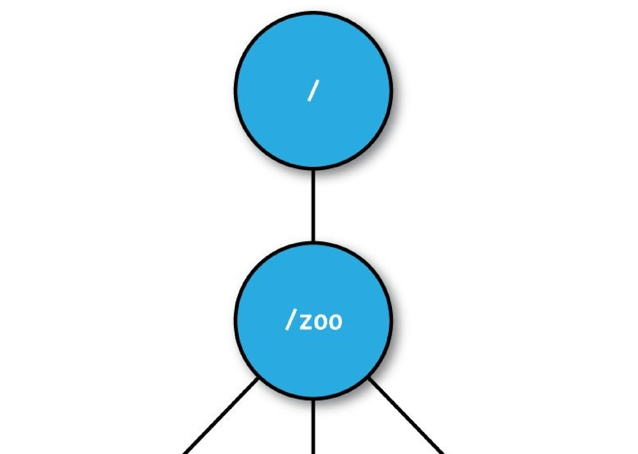
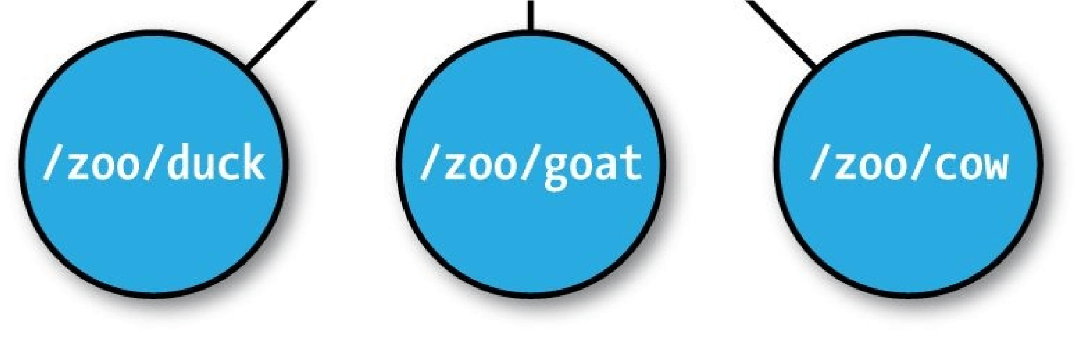
Figure 21-1. ZooKeeper znodes
In this example we won’t store data in any of the znodes, but in a real application you could imagine storing data about the members, such as hostnames, in their znodes.
Creating the Group
Let’s introduce ZooKeeper’s Java API by writing a program to create a znode for the group, which is /zoo in Example 21-1.
Example 21-1. A program to create a znode representing a group in ZooKeeper
public class CreateGroup implements Watcher {
private static final int SESSIONTIMEOUT = 5000;
private ZooKeeper zk; private CountDownLatch connectedSignal = new CountDownLatch(1);
public void connect(String hosts) throws IOException, InterruptedException { zk = new ZooKeeper(hosts, SESSION_TIMEOUT, this); connectedSignal.await();
}
@Override
public void process(WatchedEvent event) { // Watcher interface if (event.getState() == KeeperState.SyncConnected) { connectedSignal.countDown();
}
}
public void create(String groupName) throws KeeperException,
InterruptedException {
String path = “/“ + groupName;
String createdPath = zk.create(path, null/data/_, Ids.OPEN_ACL_UNSAFE, CreateMode.PERSISTENT);
System.out.println(“Created “ + createdPath);
}
public void close() throws InterruptedException { zk.close();
}
public static void main(String[] args) throws Exception { CreateGroup createGroup = new CreateGroup(); createGroup.connect(args[0]); createGroup.create(args[1]); createGroup.close();
} }
When the main() method is run, it creates a CreateGroup instance and then calls its connect() method. This method instantiates a new ZooKeeper object, which is the central class of the client API and the one that maintains the connection between the client and the ZooKeeper service. The constructor takes three arguments: the first is the host address
(and optional port, which defaults to 2181) of the ZooKeeper service;142] the second is the session timeout in milliseconds (which we set to 5 seconds), explained in more detail later; and the third is an instance of a Watcher object. The Watcher object receives callbacks from ZooKeeper to inform it of various events. In this scenario, CreateGroup is a Watcher, so we pass this to the ZooKeeper constructor.
When a ZooKeeper instance is created, it starts a thread to connect to the ZooKeeper service. The call to the constructor returns immediately, so it is important to wait for the connection to be established before using the ZooKeeper object. We make use of Java’s
CountDownLatch class (in the java.util.concurrent package) to block until the ZooKeeper instance is ready. This is where the Watcher comes in. The Watcher interface has a single method: public void process(WatchedEvent event);
When the client has connected to ZooKeeper, the Watcher receives a call to its process() method with an event indicating that it has connected. On receiving a connection event
(represented by the Watcher.Event.KeeperState enum, with value SyncConnected), we decrement the counter in the CountDownLatch, using its countDown() method. The latch was created with a count of one, representing the number of events that need to occur before it releases all waiting threads. After calling countDown() once, the counter reaches zero and the await() method returns.
The connect() method has now returned, and the next method to be invoked on the CreateGroup is the create() method. In this method, we create a new ZooKeeper znode using the create() method on the ZooKeeper instance. The arguments it takes are the path (represented by a string), the contents of the znode (a byte array null here), an access control list (or ACL for short, which here is completely open, allowing any client to read from or write to the znode), and the nature of the znode to be created.
Znodes may be ephemeral or persistent. An ephemeral znode will be deleted by the ZooKeeper service when the client that created it disconnects, either explicitly or because the client terminates for whatever reason. A persistent znode, on the other hand, is not deleted when the client disconnects. We want the znode representing a group to live longer than the lifetime of the program that creates it, so we create a persistent znode.
The return value of the create() method is the path that was created by ZooKeeper. We use it to print a message that the path was successfully created. We will see how the path returned by create() may differ from the one passed into the method when we look at sequential znodes.
To see the program in action, we need to have ZooKeeper running on the local machine, and then we can use the following:
% export CLASSPATH=ch21-zk/target/classes/:$ZOOKEEPER_HOME/*:\
$ZOOKEEPER_HOME/lib/*:$ZOOKEEPER_HOME/conf
% java CreateGroup localhost zoo Created /zoo
Joining a Group
The next part of the application is a program to register a member in a group. Each member will run as a program and join a group. When the program exits, it should be removed from the group, which we can do by creating an ephemeral znode that represents it in the ZooKeeper namespace.
The JoinGroup program implements this idea, and its listing is in Example 21-2. The logic for creating and connecting to a ZooKeeper instance has been refactored into a base class, ConnectionWatcher, and appears in Example 21-3. Example 21-2. A program that joins a group
public class JoinGroup extends ConnectionWatcher {
public void join(String groupName, String memberName) throws KeeperException,
InterruptedException {
String path = “/“ + groupName + “/“ + memberName;
String createdPath = zk.create(path, null/data/, Ids.OPENACL_UNSAFE,
CreateMode.EPHEMERAL);
System.out.println(“Created “ + createdPath);
}
public static void main(String[] args) throws Exception { JoinGroup joinGroup = new JoinGroup(); joinGroup.connect(args[0]); joinGroup.join(args[1], args[2]);
// stay alive until process is killed or thread is interrupted_
Thread.sleep(Long.MAX_VALUE);
} }
Example 21-3. A helper class that waits for the ZooKeeper connection to be established
public class ConnectionWatcher implements Watcher {
private static final int SESSION_TIMEOUT = 5000;
protected ZooKeeper zk;
private CountDownLatch connectedSignal = new CountDownLatch(1);
public void connect(String hosts) throws IOException, InterruptedException { zk = new ZooKeeper(hosts, SESSION_TIMEOUT, this); connectedSignal.await();
}
@Override
public void process(WatchedEvent event) { if (event.getState() == KeeperState.SyncConnected) { connectedSignal.countDown();
}
}
public void close() throws InterruptedException { zk.close();
} }
The code for JoinGroup is very similar to CreateGroup. It creates an ephemeral znode as a child of the group znode in its join() method, then simulates doing work of some kind by sleeping until the process is forcibly terminated. Later, you will see that upon termination, the ephemeral znode is removed by ZooKeeper.
Listing Members in a Group
Now we need a program to find the members in a group (see Example 21-4). Example 21-4. A program to list the members in a group
public class ListGroup extends ConnectionWatcher { public void list(String groupName) throws KeeperException,
InterruptedException {
String path = “/“ + groupName;
try {
List
System.out.printf(“No members in group %s\n”, groupName);
System.exit(1);
}
for (String child : children) {
System.out.println(child);
}
} catch (KeeperException.NoNodeException e) {
System.out.printf(“Group %s does not exist\n”, groupName);
System.exit(1);
}
}
public static void main(String[] args) throws Exception { ListGroup listGroup = new ListGroup(); listGroup.connect(args[0]); listGroup.list(args[1]); listGroup.close();
} }
In the list() method, we call getChildren() with a znode path and a watch flag to retrieve a list of child paths for the znode, which we print out. Placing a watch on a znode causes the registered Watcher to be triggered if the znode changes state. Although we’re not using it here, watching a znode’s children would permit a program to get notifications of members joining or leaving the group, or of the group being deleted.
We catch KeeperException.NoNodeException, which is thrown in the case when the group’s znode does not exist.
Let’s see ListGroup in action. As expected, the zoo group is empty, since we haven’t added any members yet:
% java ListGroup localhost zoo No members in group zoo
We can use JoinGroup to add some members. We launch them as background processes, since they don’t terminate on their own (due to the sleep statement):
% java JoinGroup localhost zoo duck &
% java JoinGroup localhost zoo cow &
% java JoinGroup localhost zoo goat & % goat_pid=$!
The last line saves the process ID of the Java process running the program that adds goat as a member. We need to remember the ID so that we can kill the process in a moment, after checking the members:
% java ListGroup localhost zoo goat duck cow
To remove a member, we kill its process:
% kill $goat_pid
And a few seconds later, it has disappeared from the group because the process’s ZooKeeper session has terminated (the timeout was set to 5 seconds) and its associated ephemeral node has been removed:
% java ListGroup localhost zoo
duck cow
Let’s stand back and see what we’ve built here. We have a way of building up a list of a group of nodes that are participating in a distributed system. The nodes may have no knowledge of each other. A client that wants to use the nodes in the list to perform some work, for example, can discover the nodes without them being aware of the client’s existence.
Finally, note that group membership is not a substitution for handling network errors when communicating with a node. Even if a node is a group member, communications with it may fail, and such failures must be handled in the usual ways (retrying, trying a different member of the group, etc.).
ZooKeeper command-line tools
ZooKeeper comes with a command-line tool for interacting with the ZooKeeper namespace. We can use it to list the znodes under the /zoo znode as follows:
% zkCli.sh -server localhost ls /zoo
[cow, duck]
You can run the command without arguments to display usage instructions.
Deleting a Group
To round off the example, let’s see how to delete a group. The ZooKeeper class provides a delete() method that takes a path and a version number. ZooKeeper will delete a znode only if the version number specified is the same as the version number of the znode it is trying to delete — an optimistic locking mechanism that allows clients to detect conflicts over znode modification. You can bypass the version check, however, by using a version number of –1 to delete the znode regardless of its version number.
There is no recursive delete operation in ZooKeeper, so you have to delete child znodes before parents. This is what we do in the DeleteGroup class, which will remove a group and all its members (Example 21-5).
Example 21-5. A program to delete a group and its members
public class DeleteGroup extends ConnectionWatcher {
public void delete(String groupName) throws KeeperException,
InterruptedException {
String path = “/“ + groupName;
try {
List
}
zk.delete(path, -1);
} catch (KeeperException.NoNodeException e) {
System.out.printf(“Group %s does not exist\n”, groupName);
System.exit(1);
}
}
public static void main(String[] args) throws Exception { DeleteGroup deleteGroup = new DeleteGroup(); deleteGroup.connect(args[0]); deleteGroup.delete(args[1]); deleteGroup.close(); }
}
Finally, we can delete the zoo group that we created earlier:
% java DeleteGroup localhost zoo
% java ListGroup localhost zoo Group zoo does not exist
The ZooKeeper Service
ZooKeeper is a highly available, high-performance coordination service. In this section, we look at the nature of the service it provides: its model, operations, and implementation.
Data Model
ZooKeeper maintains a hierarchical tree of nodes called znodes. A znode stores data and has an associated ACL. ZooKeeper is designed for coordination (which typically uses small datafiles), not high-volume data storage, so there is a limit of 1 MB on the amount of data that may be stored in any znode.
Data access is atomic. A client reading the data stored in a znode will never receive only some of the data; either the data will be delivered in its entirety or the read will fail. Similarly, a write will replace all the data associated with a znode. ZooKeeper guarantees that the write will either succeed or fail; there is no such thing as a partial write, where only some of the data written by the client is stored. ZooKeeper does not support an append operation. These characteristics contrast with HDFS, which is designed for highvolume data storage with streaming data access and provides an append operation.
Znodes are referenced by paths, which in ZooKeeper are represented as slash-delimited Unicode character strings, like filesystem paths in Unix. Paths must be absolute, so they must begin with a slash character. Furthermore, they are canonical, which means that each path has a single representation, and so paths do not undergo resolution. For example, in Unix, a file with the path /a/b can equivalently be referred to by the path /a/./b because “.” refers to the current directory at the point it is encountered in the path. In ZooKeeper, “.” does not have this special meaning and is actually illegal as a path component (as is “..” for the parent of the current directory).
Path components are composed of Unicode characters, with a few restrictions (these are spelled out in the ZooKeeper reference documentation). The string “zookeeper” is a reserved word and may not be used as a path component. In particular, ZooKeeper uses the /zookeeper subtree to store management information, such as information on quotas.
Note that paths are not URIs, and they are represented in the Java API by a java.lang.String, rather than the Hadoop Path class (or the java.net.URI class, for that matter).
Znodes have some properties that are very useful for building distributed applications, which we discuss in the following sections.
Ephemeral znodes
As we’ve seen, znodes can be one of two types: ephemeral or persistent. A znode’s type is set at creation time and may not be changed later. An ephemeral znode is deleted by ZooKeeper when the creating client’s session ends. By contrast, a persistent znode is not tied to the client’s session and is deleted only when explicitly deleted by a client (not necessarily the one that created it). An ephemeral znode may not have children, not even ephemeral ones.
Even though ephemeral nodes are tied to a client session, they are visible to all clients (subject to their ACL policies, of course).
Ephemeral znodes are ideal for building applications that need to know when certain distributed resources are available. The example earlier in this chapter uses ephemeral znodes to implement a group membership service, so any process can discover the members of the group at any particular time.
Sequence numbers
A sequential znode is given a sequence number by ZooKeeper as a part of its name. If a znode is created with the sequential flag set, then the value of a monotonically increasing counter (maintained by the parent znode) is appended to its name.
If a client asks to create a sequential znode with the name /a/b-, for example, the znode created may actually have the name /a/b-3.143] If, later on, another sequential znode with the name /a/b- is created, it will be given a unique name with a larger value of the counter — for example, /a/b-5. In the Java API, the actual path given to sequential znodes is communicated back to the client as the return value of the create() call.
Sequence numbers can be used to impose a global ordering on events in a distributed system and may be used by the client to infer the ordering. In A Lock Service, you will learn how to use sequential znodes to build a shared lock.
Watches
Watches allow clients to get notifications when a znode changes in some way. Watches are set by operations on the ZooKeeper service and are triggered by other operations on the service. For example, a client might call the exists operation on a znode, placing a watch on it at the same time. If the znode doesn’t exist, the exists operation will return false. If, some time later, the znode is created by a second client, the watch is triggered, notifying the first client of the znode’s creation. You will see precisely which operations trigger others in the next section.
Watchers are triggered only once.144] To receive multiple notifications, a client needs to reregister the watch. So, if the client in the previous example wishes to receive further notifications for the znode’s existence (to be notified when it is deleted, for example), it needs to call the exists operation again to set a new watch.
There is an example in A Configuration Service demonstrating how to use watches to update configuration across a cluster.
Operations
There are nine basic operations in ZooKeeper, listed in Table 21-2.
Table 21-2. Operations in the ZooKeeper service
Operation Description
| create | Creates a znode (the parent znode must already exist) |
|---|---|
| delete | Deletes a znode (the znode must not have any children) |
| exists | Tests whether a znode exists and retrieves its metadata |
| getACL, setACL | Gets/sets the ACL for a znode |
| getChildren | Gets a list of the children of a znode |
| getData, setData | Gets/sets the data associated with a znode |
| sync | Synchronizes a client’s view of a znode with ZooKeeper |
Update operations in ZooKeeper are conditional. A delete or setData operation has to specify the version number of the znode that is being updated (which is found from a previous exists call). If the version number does not match, the update will fail. Updates are a nonblocking operation, so a client that loses an update (because another process updated the znode in the meantime) can decide whether to try again or take some other action, and it can do so without blocking the progress of any other process.
Although ZooKeeper can be viewed as a filesystem, there are some filesystem primitives that it does away with in the name of simplicity. Because files are small and are written and read in their entirety, there is no need to provide open, close, or seek operations.
WARNING
The sync operation is not like fsync() in POSIX filesystems. As mentioned earlier, writes in ZooKeeper are atomic, and a successful write operation is guaranteed to have been written to persistent storage on a majority of ZooKeeper servers. However, it is permissible for reads to lag the latest state of the ZooKeeper service, and the sync operation exists to allow a client to bring itself up to date. This topic is covered in more detail in Consistency.
Multiupdate
There is another ZooKeeper operation, called multi, that batches together multiple primitive operations into a single unit that either succeeds or fails in its entirety. The situation where some of the primitive operations succeed and some fail can never arise.
Multiupdate is very useful for building structures in ZooKeeper that maintain some global invariant. One example is an undirected graph. Each vertex in the graph is naturally represented as a znode in ZooKeeper, and to add or remove an edge we need to update the two znodes corresponding to its vertices because each has a reference to the other. If we used only primitive ZooKeeper operations, it would be possible for another client to observe the graph in an inconsistent state, where one vertex is connected to another but the reverse connection is absent. Batching the updates on the two znodes into one multi operation ensures that the update is atomic, so a pair of vertices can never have a dangling connection.
APIs
There are two core language bindings for ZooKeeper clients, one for Java and one for C; there are also contrib bindings for Perl, Python, and REST clients. For each binding, there is a choice between performing operations synchronously or asynchronously. We’ve already seen the synchronous Java API. Here’s the signature for the exists operation, which returns either a Stat object that encapsulates the znode’s metadata or null if the znode doesn’t exist:
public Stat exists(String path, Watcher watcher) throws KeeperException, InterruptedException
The asynchronous equivalent, which is also found in the ZooKeeper class, looks like this: public void exists(String path, Watcher watcher, StatCallback cb, Object ctx)
In the Java API, all the asynchronous methods have void return types, since the result of the operation is conveyed via a callback. The caller passes a callback implementation whose method is invoked when a response is received from ZooKeeper. In this case, the callback is the StatCallback interface, which has the following method: public void processResult(int rc, String path, Object ctx, Stat stat);
The rc argument is the return code, corresponding to the codes defined by
KeeperException. A nonzero code represents an exception, in which case the stat parameter will be null. The path and ctx arguments correspond to the equivalent arguments passed by the client to the exists() method, and can be used to identify the request for which this callback is a response. The ctx parameter can be an arbitrary object that may be used by the client when the path does not give enough context to disambiguate the request. If not needed, it may be set to null.
There are actually two C shared libraries. The single-threaded library, zookeeperst, supports only the asynchronous API and is intended for platforms where the pthread library is not available or stable. Most developers will use the multithreaded library, zookeeper_mt, as it supports both the synchronous and asynchronous APIs. For details on how to build and use the C API, refer to the _README file in the src/c directory of the ZooKeeper distribution.
SHOULD I USE THE SYNCHRONOUS OR ASYNCHRONOUS API?
Both APIs offer the same functionality, so the one you use is largely a matter of style. The asynchronous API is appropriate if you have an event-driven programming model, for example.
The asynchronous API allows you to pipeline requests, which in some scenarios can offer better throughput. Imagine that you want to read a large batch of znodes and process them independently. Using the synchronous API, each read would block until it returned, whereas with the asynchronous API, you can fire off all the asynchronous reads very quickly and process the responses in a separate thread as they come back.
Watch triggers
The read operations exists, getChildren, and getData may have watches set on them, and the watches are triggered by write operations: create, delete, and setData. ACL operations do not participate in watches. When a watch is triggered, a watch event is generated, and the watch event’s type depends both on the watch and the operation that triggered it:
A watch set on an exists operation will be triggered when the znode being watched is created, deleted, or has its data updated.
A watch set on a getData operation will be triggered when the znode being watched is deleted or has its data updated. No trigger can occur on creation because the znode must already exist for the getData operation to succeed. A watch set on a getChildren operation will be triggered when a child of the znode being watched is created or deleted, or when the znode itself is deleted. You can tell whether the znode or its child was deleted by looking at the watch event type:
NodeDeleted shows the znode was deleted, and NodeChildrenChanged indicates that it was a child that was deleted.
The combinations are summarized in Table 21-3.
Table 21-3. Watch creation operations and their corresponding triggers
Watch trigger
| Watch creation create znode create child | delete znode delete child | setData |
| exists NodeCreated | NodeDeleted | NodeDataChanged |
| getData | NodeDeleted | NodeDataChanged |
getChildren NodeChildrenChanged NodeDeleted NodeChildrenChanged <br /><br />A watch event includes the path of the znode that was involved in the event, so for<br />NodeCreated and NodeDeleted events, you can tell which node was created or deleted simply by inspecting the path. To discover which children have changed after a<br />NodeChildrenChanged event, you need to call getChildren again to retrieve the new list of children. Similarly, to discover the new data for a NodeDataChanged event, you need to call getData. In both of these cases, the state of the znodes may have changed between receiving the watch event and performing the read operation, so you should bear this in mind when writing applications.
ACLs
A znode is created with a list of ACLs, which determine who can perform certain operations on it.
ACLs depend on authentication, the process by which the client identifies itself to ZooKeeper. There are a few authentication schemes that ZooKeeper provides: digest
The client is authenticated by a username and password. sasl
The client is authenticated using Kerberos. ip
The client is authenticated by its IP address.
Clients may authenticate themselves after establishing a ZooKeeper session.
Authentication is optional, although a znode’s ACL may require an authenticated client, in which case the client must authenticate itself to access the znode. Here is an example of using the digest scheme to authenticate with a username and password: zk.addAuthInfo(“digest”, “tom:secret”.getBytes());
An ACL is the combination of an authentication scheme, an identity for that scheme, and a set of permissions. For example, if we wanted to give a client with the IP address 10.0.0.1 read access to a znode, we would set an ACL on the znode with the ip scheme, an ID of 10.0.0.1, and READ permission. In Java, we would create the ACL object as follows:
new ACL(Perms.READ, new Id(“ip”, “10.0.0.1”));
The full set of permissions are listed in Table 21-4. Note that the exists operation is not governed by an ACL permission, so any client may call exists to find the Stat for a znode or to discover that a znode does not in fact exist.
Table 21-4. ACL permissions
ACL permission Permitted operations
CREATE create (a child znode)
| READ | getChildren |
|---|---|
| getData | |
| WRITE | setData |
DELETE delete (a child znode)
| ADMIN | setACL |
|---|---|
There are a number of predefined ACLs in the ZooDefs.Ids class, including
OPEN_ACL_UNSAFE, which gives all permissions (except ADMIN permission) to everyone.
In addition, ZooKeeper has a pluggable authentication mechanism, which makes it possible to integrate third-party authentication systems if needed.
Implementation
The ZooKeeper service can run in two modes. In standalone mode, there is a single ZooKeeper server, which is useful for testing due to its simplicity (it can even be embedded in unit tests) but provides no guarantees of high availability or resilience. In production, ZooKeeper runs in replicated mode on a cluster of machines called an ensemble. ZooKeeper achieves high availability through replication, and can provide a service as long as a majority of the machines in the ensemble are up. For example, in a five-node ensemble, any two machines can fail and the service will still work because a majority of three remain. Note that a six-node ensemble can also tolerate only two machines failing, because if three machines fail, the remaining three do not constitute a majority of the six. For this reason, it is usual to have an odd number of machines in an ensemble.
Conceptually, ZooKeeper is very simple: all it has to do is ensure that every modification to the tree of znodes is replicated to a majority of the ensemble. If a minority of the machines fail, then a minimum of one machine will survive with the latest state. The other remaining replicas will eventually catch up with this state.
The implementation of this simple idea, however, is nontrivial. ZooKeeper uses a protocol called Zab that runs in two phases, which may be repeated indefinitely:
Phase 1: Leader election
The machines in an ensemble go through a process of electing a distinguished member, called the leader. The other machines are termed followers. This phase is finished once a majority (or quorum) of followers have synchronized their state with the leader.
Phase 2: Atomic broadcast
All write requests are forwarded to the leader, which broadcasts the update to the followers. When a majority have persisted the change, the leader commits the update, and the client gets a response saying the update succeeded. The protocol for achieving consensus is designed to be atomic, so a change either succeeds or fails. It resembles a two-phase commit.
DOES ZOOKEEPER USE PAXOS?
No. ZooKeeper’s Zab protocol is not the same as the well-known Paxos algorithm.[145] Zab is similar, but it differs in several aspects of its operation, such as relying on TCP for its message ordering guarantees.[146]
Google’s Chubby Lock Service,[147] which shares similar goals with ZooKeeper, is based on Paxos.
If the leader fails, the remaining machines hold another leader election and continue as before with the new leader. If the old leader later recovers, it then starts as a follower. Leader election is very fast, around 200 ms according to one published result, so performance does not noticeably degrade during an election.
All machines in the ensemble write updates to disk before updating their in-memory copies of the znode tree. Read requests may be serviced from any machine, and because they involve only a lookup from memory, they are very fast.
Consistency
Understanding the basis of ZooKeeper’s implementation helps in understanding the consistency guarantees that the service makes. The terms “leader” and “follower” for the machines in an ensemble are apt because they make the point that a follower may lag the leader by a number of updates. This is a consequence of the fact that only a majority and not all members of the ensemble need to have persisted a change before it is committed. A good mental model for ZooKeeper is of clients connected to ZooKeeper servers that are following the leader. A client may actually be connected to the leader, but it has no control over this and cannot even know if this is the case.148] See Figure 21-2.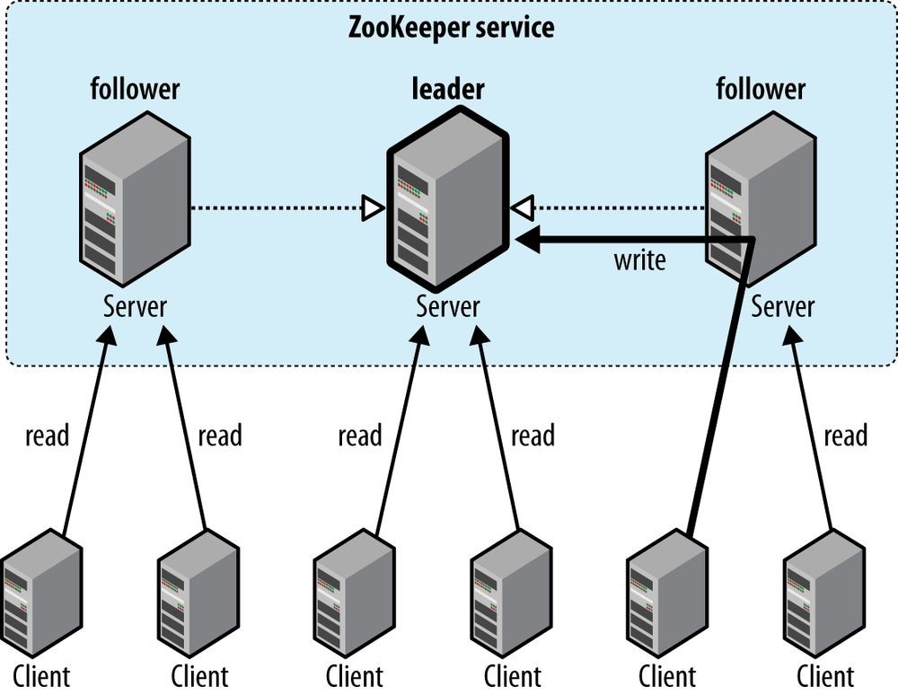
Figure 21-2. Reads are satisfied by followers, whereas writes are committed by the leader
Every update made to the znode tree is given a globally unique identifier, called a zxid (which stands for “ZooKeeper transaction ID”). Updates are ordered, so if zxid z is less than z, then z happened before z, according to ZooKeeper (which is the single authority on ordering in the distributed system).
The following guarantees for data consistency flow from ZooKeeper’s design:
Sequential consistency
Updates from any particular client are applied in the order that they are sent. This means that if a client updates the znode z to the value a, and in a later operation, it updates z to the value b, then no client will ever see z with value a after it has seen it with value b (if no other updates are made to z).
Atomicity
Updates either succeed or fail. This means that if an update fails, no client will ever see it.
Single system image
A client will see the same view of the system, regardless of the server it connects to. This means that if a client connects to a new server during the same session, it will not see an older state of the system than the one it saw with the previous server. When a server fails and a client tries to connect to another in the ensemble, a server that is behind the one that failed will not accept connections from the client until it has caught up with the failed server.
Durability
Once an update has succeeded, it will persist and will not be undone. This means updates will survive server failures.
Timeliness
The lag in any client’s view of the system is bounded, so it will not be out of date by more than some multiple of tens of seconds. This means that rather than allow a client to see data that is very stale, a server will shut down, forcing the client to switch to a more up-to-date server.
For performance reasons, reads are satisfied from a ZooKeeper server’s memory and do not participate in the global ordering of writes. This property can lead to the appearance of inconsistent ZooKeeper states from clients that communicate through a mechanism outside ZooKeeper: for example, client A updates znode z from a to a’, A tells B to read z, and B reads the value of z as a, not a’. This is perfectly compatible with the guarantees that ZooKeeper makes (the condition that it does not promise is called “simultaneously consistent cross-client views”). To prevent this condition from happening, B should call sync on z before reading z’s value. The sync operation forces the ZooKeeper server to which B is connected to “catch up” with the leader, so that when B reads z’s value, it will be the one that A set (or a later value).
NOTE
Slightly confusingly, the sync operation is available only as an asynchronous call. This is because you don’t need to wait for it to return, since ZooKeeper guarantees that any subsequent operation will happen after the sync completes on the server, even if the operation is issued before the sync completes.
Sessions
A ZooKeeper client is configured with the list of servers in the ensemble. On startup, it tries to connect to one of the servers in the list. If the connection fails, it tries another server in the list, and so on, until it either successfully connects to one of them or fails because all ZooKeeper servers are unavailable.
Once a connection has been made with a ZooKeeper server, the server creates a new session for the client. A session has a timeout period that is decided on by the application that creates it. If the server hasn’t received a request within the timeout period, it may expire the session. Once a session has expired, it may not be reopened, and any ephemeral nodes associated with the session will be lost. Although session expiry is a comparatively rare event, since sessions are long lived, it is important for applications to handle it (we will see how in The Resilient ZooKeeper Application).
Sessions are kept alive by the client sending ping requests (also known as heartbeats) whenever the session is idle for longer than a certain period. (Pings are automatically sent by the ZooKeeper client library, so your code doesn’t need to worry about maintaining the session.) The period is chosen to be low enough to detect server failure (manifested by a read timeout) and reconnect to another server within the session timeout period.
Failover to another ZooKeeper server is handled automatically by the ZooKeeper client, and crucially, sessions (and associated ephemeral znodes) are still valid after another server takes over from the failed one.
During failover, the application will receive notifications of disconnections and connections to the service. Watch notifications will not be delivered while the client is disconnected, but they will be delivered when the client successfully reconnects. Also, if the application tries to perform an operation while the client is reconnecting to another server, the operation will fail. This underlines the importance of handling connection loss exceptions in real-world ZooKeeper applications (described in The Resilient ZooKeeper Application).
Time
There are several time parameters in ZooKeeper. The tick time is the fundamental period of time in ZooKeeper and is used by servers in the ensemble to define the schedule on which their interactions run. Other settings are defined in terms of tick time, or are at least constrained by it. The session timeout, for example, may not be less than 2 ticks or more than 20. If you attempt to set a session timeout outside this range, it will be modified to fall within the range.
A common tick time setting is 2 seconds (2,000 milliseconds). This translates to an allowable session timeout of between 4 and 40 seconds.
There are a few considerations in selecting a session timeout. A low session timeout leads to faster detection of machine failure. In the group membership example, the session timeout is the time it takes for a failed machine to be removed from the group. Beware of setting the session timeout too low, however, because a busy network can cause packets to be delayed and may cause inadvertent session expiry. In such an event, a machine would appear to “flap”: leaving and then rejoining the group repeatedly in a short space of time.
Applications that create more complex ephemeral state should favor longer session timeouts, as the cost of reconstruction is higher. In some cases, it is possible to design the application so it can restart within the session timeout period and avoid session expiry. (This might be desirable to perform maintenance or upgrades.) Every session is given a unique identity and password by the server, and if these are passed to ZooKeeper while a connection is being made, it is possible to recover a session (as long as it hasn’t expired). An application can therefore arrange a graceful shutdown, whereby it stores the session identity and password to stable storage before restarting the process, retrieving the stored session identity and password, and recovering the session.
You should view this feature as an optimization that can help avoid expired sessions. It does not remove the need to handle session expiry, which can still occur if a machine fails unexpectedly, or even if an application is shut down gracefully but does not restart before its session expires, for whatever reason.
As a general rule, the larger the ZooKeeper ensemble, the larger the session timeout should be. Connection timeouts, read timeouts, and ping periods are all defined internally as a function of the number of servers in the ensemble, so as the ensemble grows, these periods decrease. Consider increasing the timeout if you experience frequent connection loss. You can monitor ZooKeeper metrics — such as request latency statistics — using
JMX.
States
The ZooKeeper object transitions through different states in its lifecycle (see Figure 21-3). You can query its state at any time by using the getState() method: public States getState()
States is an enum representing the different states that a ZooKeeper object may be in. (Despite the enum’s name, an instance of ZooKeeper may be in only one state at a time.) A newly constructed ZooKeeper instance is in the CONNECTING state while it tries to establish a connection with the ZooKeeper service. Once a connection is established, it goes into the CONNECTED state.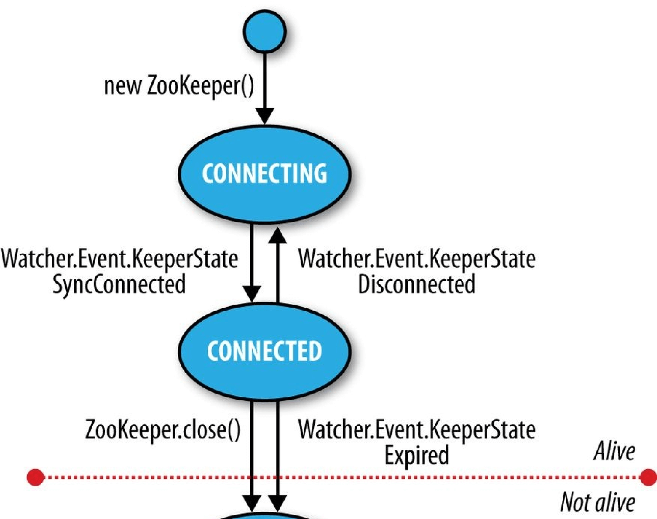

Figure 21-3. ZooKeeper state transitions
A client using the ZooKeeper object can receive notifications of the state transitions by registering a Watcher object. On entering the CONNECTED state, the watcher receives a WatchedEvent whose KeeperState value is SyncConnected.
NOTE
A ZooKeeper Watcher object serves double duty: it can be used to be notified of changes in the ZooKeeper state (as described in this section), and it can be used to be notified of changes in znodes (described in Watch triggers). The (default) watcher passed into the ZooKeeper object constructor is used for state changes, but znode changes may either use a dedicated instance of Watcher (by passing one in to the appropriate read operation) or share the default one if using the form of the read operation that takes a Boolean flag to specify whether to use a watcher.
The ZooKeeper instance may disconnect and reconnect to the ZooKeeper service, moving between the CONNECTED and CONNECTING states. If it disconnects, the watcher receives a Disconnected event. Note that these state transitions are initiated by the ZooKeeper instance itself, and it will automatically try to reconnect if the connection is lost.
The ZooKeeper instance may transition to a third state, CLOSED, if either the close() method is called or the session times out, as indicated by a KeeperState of type Expired. Once in the CLOSED state, the ZooKeeper object is no longer considered to be alive (this can be tested using the isAlive() method on States) and cannot be reused. To reconnect to the ZooKeeper service, the client must construct a new ZooKeeper instance.
Building Applications with ZooKeeper
Having covered ZooKeeper in some depth, let’s turn back to writing some useful applications with it.
A Configuration Service
One of the most basic services that a distributed application needs is a configuration service, so that common pieces of configuration information can be shared by machines in a cluster. At the simplest level, ZooKeeper can act as a highly available store for configuration, allowing application participants to retrieve or update configuration files. Using ZooKeeper watches, it is possible to create an active configuration service, where interested clients are notified of changes in configuration.
Let’s write such a service. We make a couple of assumptions that simplify the implementation (they could be removed with a little more work). First, the only configuration values we need to store are strings, and keys are just znode paths, so we use a znode to store each key-value pair. Second, there is a single client performing updates at any one time. Among other things, this model fits with the idea of a master (such as the namenode in HDFS) that wishes to update information that its workers need to follow.
We wrap the code up in a class called ActiveKeyValueStore:
public class ActiveKeyValueStore extends ConnectionWatcher { private static final Charset CHARSET = Charset.forName(“UTF-8”);
public void write(String path, String value) throws InterruptedException,
KeeperException {
Stat stat = zk.exists(path, false); if (stat == null) { zk.create(path, value.getBytes(CHARSET), Ids.OPEN_ACL_UNSAFE,
CreateMode.PERSISTENT);
} else {
zk.setData(path, value.getBytes(CHARSET), -1); }
} }
The contract of the write() method is that a key with the given value is written to ZooKeeper. It hides the difference between creating a new znode and updating an existing znode with a new value by testing first for the znode using the exists operation and then performing the appropriate operation. The other detail worth mentioning is the need to convert the string value to a byte array, for which we just use the getBytes() method with a UTF-8 encoding.
To illustrate the use of the ActiveKeyValueStore, consider a ConfigUpdater class that updates a configuration property with a value. The listing appears in Example 21-6.
Example 21-6. An application that updates a property in ZooKeeper at random times
public class ConfigUpdater {
public static final String PATH = “/config”;
private ActiveKeyValueStore store; private Random random = new Random();
public ConfigUpdater(String hosts) throws IOException, InterruptedException { store = new ActiveKeyValueStore(); store.connect(hosts);
}
public void run() throws InterruptedException, KeeperException { while (true) {
String value = random.nextInt(100) + “”; store.write(PATH, value);
System.out.printf(“Set %s to %s\n”, PATH, value);
TimeUnit.SECONDS.sleep(random.nextInt(10));
}
}
public static void main(String[] args) throws Exception { ConfigUpdater configUpdater = new ConfigUpdater(args[0]); configUpdater.run();
} }
The program is simple. A ConfigUpdater has an ActiveKeyValueStore that connects to ZooKeeper in the ConfigUpdater’s constructor. The run() method loops forever, updating the /config znode at random times with random values.
Next, let’s look at how to read the /config configuration property. First, we add a read method to ActiveKeyValueStore:
public String read(String path, Watcher watcher) throws InterruptedException, KeeperException {
byte[] data = zk.getData(path, watcher, null/stat/); return new String(data, CHARSET); }
The getData() method of ZooKeeper takes the path, a Watcher, and a Stat object. The Stat object is filled in with values by getData() and is used to pass information back to the caller. In this way, the caller can get both the data and the metadata for a znode, although in this case, we pass a null Stat because we are not interested in the metadata.
As a consumer of the service, ConfigWatcher (see Example 21-7) creates an
ActiveKeyValueStore and, after starting, calls the store’s read() method (in its displayConfig() method) to pass a reference to itself as the watcher. It displays the initial value of the configuration that it reads.
Example 21-7. An application that watches for updates of a property in ZooKeeper and prints them to the console
public class ConfigWatcher implements Watcher {
private ActiveKeyValueStore store;
public ConfigWatcher(String hosts) throws IOException, InterruptedException { store = new ActiveKeyValueStore(); store.connect(hosts);
}
public void displayConfig() throws InterruptedException, KeeperException {
String value = store.read(ConfigUpdater.PATH, this);
System.out.printf(“Read %s as %s\n”, ConfigUpdater.PATH, value); }
@Override
public void process(WatchedEvent event) { if (event.getType() == EventType.NodeDataChanged) { try { displayConfig();
} catch (InterruptedException e) {
System.err.println(“Interrupted. Exiting.”);
Thread.currentThread().interrupt();
} catch (KeeperException e) {
System.err.printf(“KeeperException: %s. Exiting.\n”, e);
}
}
}
public static void main(String[] args) throws Exception { ConfigWatcher configWatcher = new ConfigWatcher(args[0]); configWatcher.displayConfig();
// stay alive until process is killed or thread is interrupted
Thread.sleep(Long.MAX_VALUE);
} }
When the ConfigUpdater updates the znode, ZooKeeper causes the watcher to fire with an event type of EventType.NodeDataChanged. ConfigWatcher acts on this event in its process() method by reading and displaying the latest version of the config.
Because watches are one-time signals, we tell ZooKeeper of the new watch each time we call read() on ActiveKeyValueStore, which ensures we see future updates. We are not guaranteed to receive every update, though, because the znode may have been updated (possibly many times) during the span of time between the receipt of the watch event and the next read, and as the client has no watch registered during that period, it is not notified. For the configuration service, this is not a problem, because clients care only about the latest value of a property, as it takes precedence over previous values. However, in general you should be aware of this potential limitation.
Let’s see the code in action. Launch the ConfigUpdater in one terminal window:
% java ConfigUpdater localhost
Set /config to 79
Set /config to 14
Set /config to 78
Then launch the ConfigWatcher in another window immediately afterward:
% java ConfigWatcher localhost
Read /config as 79
Read /config as 14
Read /config as 78
The Resilient ZooKeeper Application
The first of the Fallacies of Distributed Computing states that “the network is reliable.” As they stand, our programs so far have been assuming a reliable network, so when they run on a real network, they can fail in several ways. Let’s examine some possible failure modes and what we can do to correct them so that our programs are resilient in the face of failure.
Every ZooKeeper operation in the Java API declares two types of exception in its throws clause: InterruptedException and KeeperException.
InterruptedException
An InterruptedException is thrown if the operation is interrupted. There is a standard Java mechanism for canceling blocking methods, which is to call interrupt() on the thread from which the blocking method was called. A successful cancellation will result in an InterruptedException. ZooKeeper adheres to this standard, so you can cancel a ZooKeeper operation in this way. Classes or libraries that use ZooKeeper usually should propagate the InterruptedException so that their clients can cancel their operations.149] An InterruptedException does not indicate a failure, but rather that the operation has been canceled, so in the configuration application example it is appropriate to propagate the exception, causing the application to terminate.
KeeperException
A KeeperException is thrown if the ZooKeeper server signals an error or if there is a communication problem with the server. For different error cases, there are various subclasses of KeeperException. For example, KeeperException.NoNodeException is a subclass of KeeperException that is thrown if you try to perform an operation on a znode that doesn’t exist.
Every subclass of KeeperException has a corresponding code with information about the type of error. For example, for KeeperException.NoNodeException, the code is KeeperException.Code.NONODE (an enum value).
There are two ways, then, to handle KeeperException: either catch KeeperException and test its code to determine what remedying action to take, or catch the equivalent KeeperException subclasses and perform the appropriate action in each catch block.
KeeperExceptions fall into three broad categories.
State exceptions
A state exception occurs when the operation fails because it cannot be applied to the znode tree. State exceptions usually happen because another process is mutating a znode at the same time. For example, a setData operation with a version number will fail with a KeeperException.BadVersionException if the znode is updated by another process first because the version number does not match. The programmer is usually aware that this kind of conflict is possible and will code to deal with it.
Some state exceptions indicate an error in the program, such as
KeeperException.NoChildrenForEphemeralsException, which is thrown when trying to create a child znode of an ephemeral znode.
Recoverable exceptions
Recoverable exceptions are those from which the application can recover within the same
ZooKeeper session. A recoverable exception is manifested by
KeeperException.ConnectionLossException, which means that the connection to ZooKeeper has been lost. ZooKeeper will try to reconnect, and in most cases the reconnection will succeed and ensure that the session is intact.
However, ZooKeeper cannot tell if the operation that failed with a
KeeperException.ConnectionLossException was applied. This is an example of partial failure (which we introduced at the beginning of the chapter). The onus is therefore on the programmer to deal with the uncertainty, and the action that should be taken depends on the application.
At this point, it is useful to make a distinction between idempotent and _nonidempotent _operations. An idempotent operation is one that may be applied one or more times with the same result, such as a read request or an unconditional setData. These can simply be retried.
A nonidempotent operation cannot be retried indiscriminately, as the effect of applying it multiple times is not the same as that of applying it once. The program needs a way of detecting whether its update was applied by encoding information in the znode’s pathname or its data. We discuss how to deal with failed nonidempotent operations in Recoverable exceptions, when we look at the implementation of a lock service.
Unrecoverable exceptions
In some cases, the ZooKeeper session becomes invalid — perhaps because of a timeout or because the session was closed (both of these scenarios get a
KeeperException.SessionExpiredException), or perhaps because authentication failed
(KeeperException.AuthFailedException). In any case, all ephemeral nodes associated with the session will be lost, so the application needs to rebuild its state before reconnecting to ZooKeeper.
A reliable configuration service
Going back to the write() method in ActiveKeyValueStore, recall that it is composed of an exists operation followed by either a create or a setData:
public void write(String path, String value) throws InterruptedException,
KeeperException {
Stat stat = zk.exists(path, false); if (stat == null) { zk.create(path, value.getBytes(CHARSET), Ids.OPENACL_UNSAFE,
CreateMode.PERSISTENT);
} else {
zk.setData(path, value.getBytes(CHARSET), -1);
} }
Taken as a whole, the write() method is idempotent, so we can afford to unconditionally retry it. Here’s a modified version of the write() method that retries in a loop. It is set to try a maximum number of retries (MAX_RETRIES) and sleeps for RETRY_PERIOD_SECONDS between each attempt:
public void write(String path, String value) throws InterruptedException,
KeeperException { int retries = 0; while (true) { try {
Stat stat = zk.exists(path, false); if (stat == null) { zk.create(path, value.getBytes(CHARSET), Ids.OPEN_ACL_UNSAFE,
CreateMode.PERSISTENT);
} else {
zk.setData(path, value.getBytes(CHARSET), stat.getVersion());
} return;
} catch (KeeperException.SessionExpiredException e) { throw e;
} catch (KeeperException e) { if (retries++ == MAX_RETRIES) { throw e;
}
// sleep then retry
TimeUnit.SECONDS.sleep(RETRY_PERIOD_SECONDS);
}
} }
The code is careful not to retry KeeperException.SessionExpiredException, because when a session expires, the ZooKeeper object enters the CLOSED state, from which it can never reconnect (refer to Figure 21-3). We simply rethrow the exception150] and let the caller create a new ZooKeeper instance, so that the whole write() method can be retried. A simple way to create a new instance is to create a new ConfigUpdater (which we’ve actually renamed ResilientConfigUpdater) to recover from an expired session:
public static void main(String[] args) throws Exception { while (true) { try {
ResilientConfigUpdater configUpdater = new ResilientConfigUpdater(args[0]); configUpdater.run();
} **catch (KeeperException.SessionExpiredException e) {
// start a new session
} catch (KeeperException e) { // already retried, so exit_
e.printStackTrace(); break;
}
}
}
An alternative way of dealing with session expiry would be to look for a KeeperState of type Expired in the watcher (that would be the ConnectionWatcher in the example here), and create a new connection when this is detected. This way, we would just keep retrying the write() method, even if we got a KeeperException.SessionExpiredException, since the connection should eventually be reestablished. Regardless of the precise mechanics of how we recover from an expired session, the important point is that it is a different kind of failure from connection loss and needs to be handled differently.
NOTE**
There’s actually another failure mode that we’ve ignored here. When the ZooKeeper object is created, it tries to connect to a ZooKeeper server. If the connection fails or times out, then it tries another server in the ensemble. If, after trying all of the servers in the ensemble, it can’t connect, then it throws an IOException. The likelihood of all ZooKeeper servers being unavailable is low; nevertheless, some applications may choose to retry the operation in a loop until ZooKeeper is available.
This is just one strategy for retry handling. There are many others, such as using exponential backoff, where the period between retries is multiplied by a constant each time.
A Lock Service
A distributed lock is a mechanism for providing mutual exclusion between a collection of processes. At any one time, only a single process may hold the lock. Distributed locks can be used for leader election in a large distributed system, where the leader is the process that holds the lock at any point in time.
NOTE
Do not confuse ZooKeeper’s own leader election with a general leader election service, which can be built using ZooKeeper primitives (and in fact, one implementation is included with ZooKeeper). ZooKeeper’s own leader election is not exposed publicly, unlike the type of general leader election service we are describing here, which is designed to be used by distributed systems that need to agree upon a master process.
To implement a distributed lock using ZooKeeper, we use sequential znodes to impose an order on the processes vying for the lock. The idea is simple: first, designate a lock znode, typically describing the entity being locked on (say, /leader); then, clients that want to acquire the lock create sequential ephemeral znodes as children of the lock znode. At any point in time, the client with the lowest sequence number holds the lock. For example, if two clients create the znodes at /leader/lock-1 and /leader/lock-2 around the same time, then the client that created /leader/lock-1 holds the lock, since its znode has the lowest sequence number. The ZooKeeper service is the arbiter of order because it assigns the sequence numbers.
The lock may be released simply by deleting the znode /leader/lock-1; alternatively, if the client process dies, it will be deleted by virtue of being an ephemeral znode. The client that created /leader/lock-2 will then hold the lock because it has the next lowest sequence number. It ensures it will be notified that it has the lock by creating a watch that fires when znodes go away.
The pseudocode for lock acquisition is as follows:
1. Create an ephemeral sequential znode named lock- under the lock znode, and remember its actual pathname (the return value of the create operation).
2. Get the children of the lock znode and set a watch.
3. If the pathname of the znode created in step 1 has the lowest number of the children returned in step 2, then the lock has been acquired. Exit.
4. Wait for the notification from the watch set in step 2, and go to step 2.
The herd effect
Although this algorithm is correct, there are some problems with it. The first problem is that this implementation suffers from the herd effect. Consider hundreds or thousands of clients, all trying to acquire the lock. Each client places a watch on the lock znode for changes in its set of children. Every time the lock is released or another process starts the lock acquisition process, the watch fires, and every client receives a notification. The “herd effect” refers to a large number of clients being notified of the same event when only a small number of them can actually proceed. In this case, only one client will successfully acquire the lock, and the process of maintaining and sending watch events to all clients causes traffic spikes, which put pressure on the ZooKeeper servers.
To avoid the herd effect, the condition for notification needs to be refined. The key observation for implementing locks is that a client needs to be notified only when the child znode with the previous sequence number goes away, not when any child znode is deleted
(or created). In our example, if clients have created the znodes /leader/lock-1, /leader/lock-2, and /leader/lock-3, then the client holding /leader/lock-3 needs to be notified only when /leader/lock-2 disappears. It does not need to be notified when /leader/lock-1 disappears or when a new znode, /leader/lock-4, is added.
Recoverable exceptions
Another problem with the lock algorithm as it stands is that it doesn’t handle the case when the create operation fails due to connection loss. Recall that in this case we do not know whether the operation succeeded or failed. Creating a sequential znode is a nonidempotent operation, so we can’t simply retry, because if the first create had succeeded we would have an orphaned znode that would never be deleted (until the client session ended, at least). Deadlock would be the unfortunate result.
The problem is that after reconnecting, the client can’t tell whether it created any of the child znodes. By embedding an identifier in the znode name, if it suffers a connection loss, it can check to see whether any of the children of the lock node have its identifier in their names. If a child contains its identifier, it knows that the create operation succeeded, and it shouldn’t create another child znode. If no child has the identifier in its name, the client can safely create a new sequential child znode.
The client’s session identifier is a long integer that is unique for the ZooKeeper service and therefore ideal for the purpose of identifying a client across connection loss events. The session identifier can be obtained by calling the getSessionId() method on the ZooKeeper Java class.
The ephemeral sequential znode should be created with a name of the form lock__
Unrecoverable exceptions
If a client’s ZooKeeper session expires, the ephemeral znode created by the client will be deleted, effectively relinquishing the lock (or at least forfeiting the client’s turn to acquire the lock). The application using the lock should realize that it no longer holds the lock, clean up its state, and then start again by creating a new lock object and trying to acquire it. Notice that it is the application that controls this process, not the lock implementation, since it cannot second-guess how the application needs to clean up its state.
Implementation
Accounting for all of the failure modes is nontrivial, so implementing a distributed lock correctly is a delicate matter. ZooKeeper comes with a production-quality lock implementation in Java called WriteLock that is very easy for clients to use.
More Distributed Data Structures and Protocols
There are many distributed data structures and protocols that can be built with ZooKeeper, such as barriers, queues, and two-phase commit. One interesting thing to note is that these are synchronous protocols, even though we use asynchronous ZooKeeper primitives (such as notifications) to build them.
The ZooKeeper website describes several such data structures and protocols in pseudocode. ZooKeeper comes with implementations of some of these standard recipes (including locks, leader election, and queues); they can be found in the recipes directory of the distribution.
The Apache Curator project also provides an extensive set of ZooKeeper recipes, as well as a simplified ZooKeeper client.
BookKeeper and Hedwig
BookKeeper is a highly available and reliable logging service. It can be used to provide write-ahead logging, which is a common technique for ensuring data integrity in storage systems. In a system using write-ahead logging, every write operation is written to the transaction log before it is applied. Using this procedure, we don’t have to write the data to permanent storage after every write operation, because in the event of a system failure, the latest state may be recovered by replaying the transaction log for any writes that were not applied.
BookKeeper clients create logs called ledgers, and each record appended to a ledger is called a ledger entry, which is simply a byte array. Ledgers are managed by bookies, which are servers that replicate the ledger data. Note that ledger data is not stored in ZooKeeper; only metadata is.
Traditionally, the challenge has been to make systems that use write-ahead logging robust in the face of failure of the node writing the transaction log. This is usually done by replicating the transaction log in some manner. HDFS high availability, described , uses a group of journal nodes to provide a highly available edit log. Although it is similar to BookKeeper, it is a dedicated service written for HDFS, and it doesn’t use ZooKeeper as the coordination engine.
Hedwig is a topic-based ipublish-subscribe system built on BookKeeper. Thanks to its ZooKeeper underpinnings, Hedwig is a highly available service and guarantees message delivery even if subscribers are offline for extended periods of time.
BookKeeper is a ZooKeeper subproject, and you can find more information on how to use it, as well as Hedwig, at http://zookeeper.apache.org/bookkeeper/.
ZooKeeper in Production
In production, you should run ZooKeeper in replicated mode. Here, we will cover some of the considerations for running an ensemble of ZooKeeper servers. However, this section is not exhaustive, so you should consult the ZooKeeper Administrator’s Guide for detailed, up-to-date instructions, including supported platforms, recommended hardware, maintenance procedures, dynamic reconfiguration (to change the servers in a running ensemble), and configuration properties.
Resilience and Performance
ZooKeeper machines should be located to minimize the impact of machine and network failure. In practice, this means that servers should be spread across racks, power supplies, and switches, so that the failure of any one of these does not cause the ensemble to lose a majority of its servers.
For applications that require low-latency service (on the order of a few milliseconds), it is important to run all the servers in an ensemble in a single data center. Some use cases don’t require low-latency responses, however, which makes it feasible to spread servers across data centers (at least two per data center) for extra resilience. Example applications in this category are leader election and distributed coarse-grained locking, both of which have relatively infrequent state changes, so the overhead of a few tens of milliseconds incurred by inter-data-center messages is not significant relative to the overall functioning of the service.
NOTE
ZooKeeper has the concept of an observer node, which is like a non-voting follower. Because they do not participate in the vote for consensus during write requests, observers allow a ZooKeeper cluster to improve read performance without hurting write performance.[151] Observers can be used to good advantage to allow a ZooKeeper cluster to span data centers without impacting latency as much as regular voting followers. This is achieved by placing the voting members in one data center and observers in the other.
ZooKeeper is a highly available system, and it is critical that it can perform its functions in a timely manner. Therefore, ZooKeeper should run on machines that are dedicated to ZooKeeper alone. Having other applications contend for resources can cause ZooKeeper’s performance to degrade significantly.
Configure ZooKeeper to keep its transaction log on a different disk drive from its snapshots. By default, both go in the directory specified by the dataDir property, but if you specify a location for dataLogDir, the transaction log will be written there. By having its own dedicated device (not just a partition), a ZooKeeper server can maximize the rate at which it writes log entries to disk, which it does sequentially without seeking. Because all writes go through the leader, write throughput does not scale by adding servers, so it is crucial that writes are as fast as possible.
If the process swaps to disk, performance will be adversely affected. This can be avoided by setting the Java heap size to less than the amount of unused physical memory on the machine. From its configuration directory, the ZooKeeper scripts will source a file called java.env, which can be used to set the JVMFLAGS environment variable to specify the heap size (and any other desired JVM arguments).
Configuration
Each server in the ensemble of ZooKeeper servers has a numeric identifier that is unique within the ensemble and must fall between 1 and 255. The server number is specified in plain text in a file named myid in the directory specified by the dataDir property.
Setting each server number is only half of the job. We also need to give every server all the identities and network locations of the others in the ensemble. The ZooKeeper configuration file must include a line for each server, of the form: server.n=hostname:port:port
The value of n is replaced by the server number. There are two port settings: the first is the port that followers use to connect to the leader, and the second is used for leader election. Here is a sample configuration for a three-machine replicated ZooKeeper ensemble:
tickTime=2000 dataDir=/disk1/zookeeper dataLogDir=/disk2/zookeeper clientPort=2181 initLimit=5 syncLimit=2 server.1=zookeeper1:2888:3888 server.2=zookeeper2:2888:3888 server.3=zookeeper3:2888:3888
Servers listen on three ports: 2181 for client connections; 2888 for follower connections, if they are the leader; and 3888 for other server connections during the leader election phase. When a ZooKeeper server starts up, it reads the myid file to determine which server it is, and then reads the configuration file to determine the ports it should listen on and to discover the network addresses of the other servers in the ensemble.
Clients connecting to this ZooKeeper ensemble should use zookeeper1:2181,zookeeper2:2181,zookeeper3:2181 as the host string in the constructor for the ZooKeeper object.
In replicated mode, there are two extra mandatory properties: initLimit and syncLimit, both measured in multiples of tickTime.
initLimit is the amount of time to allow for followers to connect to and sync with the leader. If a majority of followers fail to sync within this period, the leader renounces its leadership status and another leader election takes place. If this happens often (and you can discover if this is the case because it is logged), it is a sign that the setting is too low.
syncLimit is the amount of time to allow a follower to sync with the leader. If a follower fails to sync within this period, it will restart itself. Clients that were attached to this follower will connect to another one.
These are the minimum settings needed to get up and running with a cluster of ZooKeeper servers. There are, however, more configuration options, particularly for tuning performance, which are documented in the ZooKeeper Administrator’s Guide.
Further Reading
For more in-depth information about ZooKeeper, see ZooKeeper by Flavio Junqueira and Benjamin Reed (O’Reilly, 2013).
[140] This is the message of Jim Waldo et al. in “A Note on Distributed Computing” (Sun Microsystems, November 1994). Distributed programming is fundamentally different from local programming, and the differences cannot simply be papered over.
[141] Detailed benchmarks are available in the excellent paper “ZooKeeper: Wait-free coordination for Internet-scale systems,” by Patrick Hunt et al. (USENIX Annual Technology Conference, 2010).
[142] For a replicated ZooKeeper service, this parameter is the comma-separated list of servers (host and optional port) in the ensemble.
[143] It is conventional (but not required) to have a trailing dash on pathnames for sequential nodes, to make their sequence numbers easy to read and parse (by the application).
[144] Except for callbacks for connection events, which do not need reregistration.
[145] Leslie Lamport, “Paxos Made Simple,” ACM SIGACT News December 2001.
[146] Zab is described in Benjamin Reed and Flavio Junqueira’s “A simple totally ordered broadcast protocol,” LADIS ’08 Proceedings of the 2nd Workshop on Large-Scale Distributed Systems and Middleware, 2008.
[147] Mike Burrows, “The Chubby Lock Service for Loosely-Coupled Distributed Systems,” November 2006.
[148] It is possible to configure ZooKeeper so that the leader does not accept client connections. In this case, its only job is to coordinate updates. Do this by setting the leaderServes property to no. This is recommended for ensembles of more than three servers.
[149] For more detail, see the excellent article “Java theory and practice: Dealing with InterruptedException” by Brian Goetz (IBM, May 2006).
[150] Another way of writing the code would be to have a single catch block, just for KeeperException, and a test to see whether its code has the value KeeperException.Code.SESSIONEXPIRED. They both behave in the same way, so which method you use is simply a matter of style.
[151] This is discussed in more detail in “Observers: Making ZooKeeper Scale Even Further” by Henry Robinson (Cloudera, December 2009).
Part V. Case Studies

若有收获,就点个赞吧
0 人点赞
